Interpreting functional-gaze and workflow figures
Plots make otherwise abstract functional estimands inspectable, but graphical smoothness is not evidence of correct specification, validated uncertainty, predictive performance, or causal identification. All figures below are built from deterministic synthetic demonstration inputs, regenerated on the documentation runner.
Units and demonstration provenance
The FPCA and function-on-scalar examples use simulate_planar_trajectories(): 2.0 seconds of synthetic trial time and normalized x/y coordinates in [0, 1] (coordinate_system="normalized", time_unit="s"). The functional regression coefficient is expressed in normalized-coordinate units per one-unit change in the synthetic continuous predictor; it is not a physical visual angle or a participant-level experimental contrast. The separate recurrence example uses an arbitrary-unit synthetic signal sampled at 0.01-second intervals. Its recurrence matrix axes refer to reconstructed-state sample indices, not screen pixels or elapsed-time values. Interpret every legend and axis within its originating fixture's units.
1. Functional principal components: variation, not a named behavior
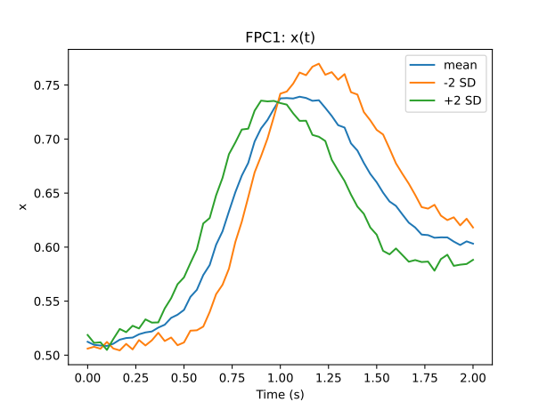
A component plot depicts a fitted direction of functional variability around the estimated mean, for an explicitly selected component and coordinate. Its sign is arbitrary; nearly tied eigenvalues can rotate the associated subspace. A visually prominent mode does not automatically map to a psychological construct such as exploration or vigilance.
Report the coordinate/time units, scaling rule, retained-rank rule, variance explained, alignment method when fits are compared, and participant-aware stability/uncertainty checks where required. Start with the FPCA guide, subspace stability and component uncertainty.
2. Functional regression: a coefficient is not a proof of significance
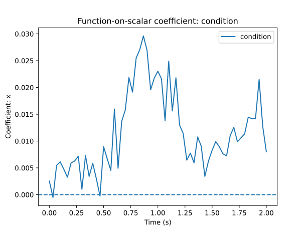
The observed-grid coefficient function describes an estimated association between the declared predictor and a functional outcome at each observation time (under the stated linear model). The displayed demonstration coefficient does not include a separately validated simultaneous confidence band. Pointwise fluctuations must not be translated into post-hoc time windows of significance.
For inferential claims, declare the hypothesis family and resampling unit, use a justified simultaneous-inference contract, and consider participant/trial dependence. Start with function-on-scalar, functional mixed effects, and whole-function inference.
3. Recurrence: dependence on declared nonlinear parameters
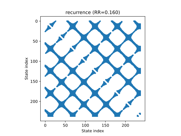
Each marked location corresponds to a pair of reconstructed states satisfying the predeclared distance threshold. Patterning depends on embedding dimension, delay, metric, radius, Theiler exclusion and minimum line lengths. It does not diagnose a unique dynamical mechanism, nor does it demonstrate causation or treatment effects.
Report the complete parameter tuple, support, recurrence rate, software conventions and defensible sensitivity analyses. Start with recurrence, threshold diagnostics, and RQA dependence.
4. Audit figures: traceability, not a quality score
- Provenance sources
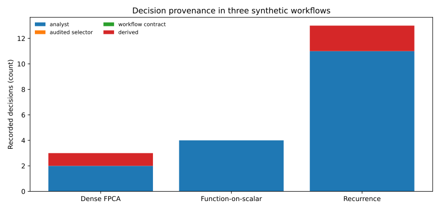
The stacked counts are derived from decisions attached to one synthetic FPCA, one function-on-scalar, and one recurrence result. More records do not imply a better or worse method. They show which choices were attributed to the analyst, selector, contract or derivation.
- Ordered step trace
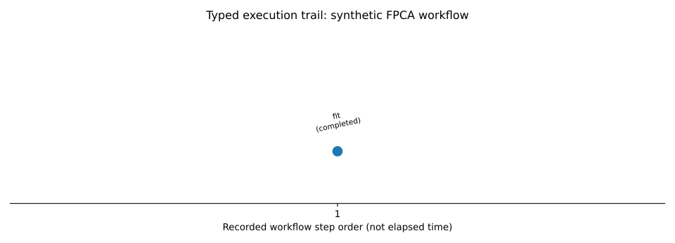
This chart displays order and recorded completion status for the synthetic FPCA example. It is not a time series, numerical benchmark, causal graph or representation of the scientific covariance.
Checklist before reproducing a figure in a manuscript
- Specify observation origin and units, number of participants/trials, and whether results are synthetic or empirical.
- State the exact quantity plotted and whether uncertainty bands are pointwise, simultaneous, conditional or fitted-model approximations.
- Record all model, bandwidth, PSD, calibration, embedding and resampling choices relevant to the figure.
- Ensure that claims do not extend beyond the fitted estimand or the design.
- Retain the code, version, audit frames, and checksummed workflow bundle.
The complete reproducible gallery also includes sparse covariance surfaces, native-support diagnostics, score uncertainty and other plot families.