Auditable Binocular Pupil Reconstruction and Sensitivity Analysis • gp3tools

Why a separate reconstruction workflow?

Binocular pupil channels are related but not interchangeable. A tracker may temporarily retain one eye while the other eye is unavailable, and a simple sample-wise mean can therefore change its measurement basis from two eyes to one without making that change visible in the analysis table. Conversely, filling a missing eye with a prediction can increase continuity while introducing model error.

gp3tools already provides lightweight binocular fusion with combine_gazepoint_eyes(), a regression-oriented fusion helper with regress_gazepoint_pupils(), pupil artifact detection, PCHIP interpolation, baseline correction, preprocessing audits, and sensitivity workflows. The functions in this article add a stricter layer for model-based missing-eye reconstruction. Their design principle is simple: a predicted pupil value must never become indistinguishable from an observed pupil value.

The workflow was motivated in part by Ong et al. (2025), who reconstructed a missing left or right pupil value from the other eye with linear regression when estimating a mean pupil series. Their paper also makes clear that regression can introduce bias when pupil variation is rapid or irregular. gp3tools therefore treats cross-eye reconstruction as a declared policy that should be validated and sensitivity-checked, not as a universally correct replacement for missing measurements.

What reconstruction does and does not mean

The workflow can estimate a temporarily unavailable pupil channel from the simultaneously observed contralateral channel. It can answer questions such as:

how much bilateral information is actually available;
whether a participant/session has enough paired samples for calibration;
how accurately an eye can be predicted when its true value is deliberately hidden;
how much of a final analysis series depends on predicted values;
whether reconstruction is concentrated in one experimental condition;
whether conclusions are sensitive to using complete cases, available-eye values, or regression-supported reconstruction.

It does not establish that a predicted value is the unobserved biological truth, that naturally missing values are missing at random, or that a high cross-eye correlation is sufficient evidence for unrestricted imputation.

Synthetic example

The example is generated entirely in R and is not an empirical Gazepoint recording. We start with simulate_gazepoint_pupil_data() and introduce short monocular losses while retaining the generator’s bilateral blink losses.

pupil <- simulate_gazepoint_pupil_data(
  n_subjects = 6,
  n_trials = 4,
  n_time_bins = 120,
  seed = 20260817
)

# Add a small deterministic between-eye calibration offset.
pupil$pupil_right <- 0.08 + 0.98 * pupil$pupil_right

# Introduce synthetic monocular losses. These are deliberately not labelled as blinks.
left_loss <- c(80:84, 510:515, 1320:1324, 2110:2116)
right_loss <- c(260:264, 890:894, 1690:1694, 2480:2485)
pupil$pupil_left[left_loss] <- NA_real_
pupil$pupil_right[right_loss] <- NA_real_

pupil[75:90, c(
  "subject", "trial", "condition", "timestamp_ms",
  "pupil_left", "pupil_right", "blink"
)]
#>    subject trial condition timestamp_ms pupil_left pupil_right blink
#> 75    S001     1   control      1233.58   3.313574    3.300916 FALSE
#> 76    S001     1   control      1250.25   3.365124    3.324580 FALSE
#> 77    S001     1   control      1266.92   3.398240    3.340684 FALSE
#> 78    S001     1   control      1283.59   3.529691    3.203018 FALSE
#> 79    S001     1   control      1300.26   3.225775    3.263195 FALSE
#> 80    S001     1   control      1316.93         NA    3.261327 FALSE
#> 81    S001     1   control      1333.60         NA    3.197705 FALSE
#> 82    S001     1   control      1350.27         NA    3.289575 FALSE
#> 83    S001     1   control      1366.94         NA    3.392627 FALSE
#> 84    S001     1   control      1383.61         NA    3.430466 FALSE
#> 85    S001     1   control      1400.28   3.531753    3.261433 FALSE
#> 86    S001     1   control      1416.95   3.167372    3.315744 FALSE
#> 87    S001     1   control      1433.62   3.321451    3.323391 FALSE
#> 88    S001     1   control      1450.29   3.241113    3.212430 FALSE
#> 89    S001     1   control      1466.96   3.395153    3.212441 FALSE
#> 90    S001     1   control      1483.63   3.286586    3.176851 FALSE

Recommended position in the preprocessing workflow

Cross-eye reconstruction and temporal interpolation address different missing-data situations. A defensible order for a study that chooses to use reconstruction is:

preserve raw eye-specific channels;
identify invalid measurements, blinks, track loss, and other artifacts;
create eye-specific cleaned channels;
diagnose bilateral availability and agreement;
fit and validate cross-eye calibration on directly observed bilateral samples;
reconstruct eligible monocular gaps, if the study has declared that policy;
construct the combined pupil signal under an explicit combination policy;
if required, interpolate remaining temporal gaps under a separately declared rule;
baseline-correct, smooth, summarise, and model;
report reconstruction burden and run sensitivity analyses.

This order is not a claim that every study should reconstruct. In many datasets the appropriate result of the diagnostic stage will be to retain available-eye or complete-case processing instead.

1. Diagnose before reconstructing

diagnostics <- diagnose_gazepoint_binocular_pupil(
  pupil,
  left_col = "pupil_left",
  right_col = "pupil_right",
  time_col = "timestamp_ms",
  group_cols = c("subject", "trial"),
  time_unit = "milliseconds",
  valid_min = 1,
  valid_max = 9,
  min_pairs = 40
)

diagnostics$summary[c(
  "subject", "trial", "n", "n_bilateral", "n_left_only",
  "n_right_only", "prop_bilateral", "correlation",
  "rmse_between_eyes", "calibration_eligible"
)]
#> # A tibble: 24 × 10
#>    subject trial     n n_bilateral n_left_only n_right_only prop_bilateral
#>    <chr>   <int> <int>       <int>       <int>        <int>          <dbl>
#>  1 S001        1   120         111           0            5          0.925
#>  2 S001        2   120         118           0            0          0.983
#>  3 S001        3   120         112           5            0          0.933
#>  4 S001        4   120         118           0            0          0.983
#>  5 S002        1   120         109           0            6          0.908
#>  6 S002        2   120         117           0            0          0.975
#>  7 S002        3   120         117           0            0          0.975
#>  8 S002        4   120         112           5            0          0.933
#>  9 S003        1   120         116           0            0          0.967
#> 10 S003        2   120         116           0            0          0.967
#> # ℹ 14 more rows
#> # ℹ 3 more variables: correlation <dbl>, rmse_between_eyes <dbl>,
#> #   calibration_eligible <lgl>

The diagnostic object also retains missing-eye run information.

head(diagnostics$gaps)
#> # A tibble: 6 × 8
#>   gap_id group_key             n_samples gap_ms edge_gap start_row end_row eye  
#>    <int> <chr>                     <int>  <dbl> <lgl>        <int>   <int> <chr>
#> 1      1 subject=S001||trial=1         1   16.7 FALSE           26      26 left 
#> 2      2 subject=S001||trial=1         2   33.3 FALSE           28      29 left 
#> 3      3 subject=S001||trial=1         5   83.4 FALSE           80      84 left 
#> 4      4 subject=S001||trial=1         1   16.7 FALSE          109     109 left 
#> 5      5 subject=S001||trial=2         1   16.7 FALSE          176     176 left 
#> 6      6 subject=S001||trial=2         1   16.7 FALSE          231     231 left

Agreement is best inspected rather than reduced to one correlation coefficient.

plot_gazepoint_binocular_diagnostics(
  pupil,
  type = "agreement",
  left_col = "pupil_left",
  right_col = "pupil_right"
)

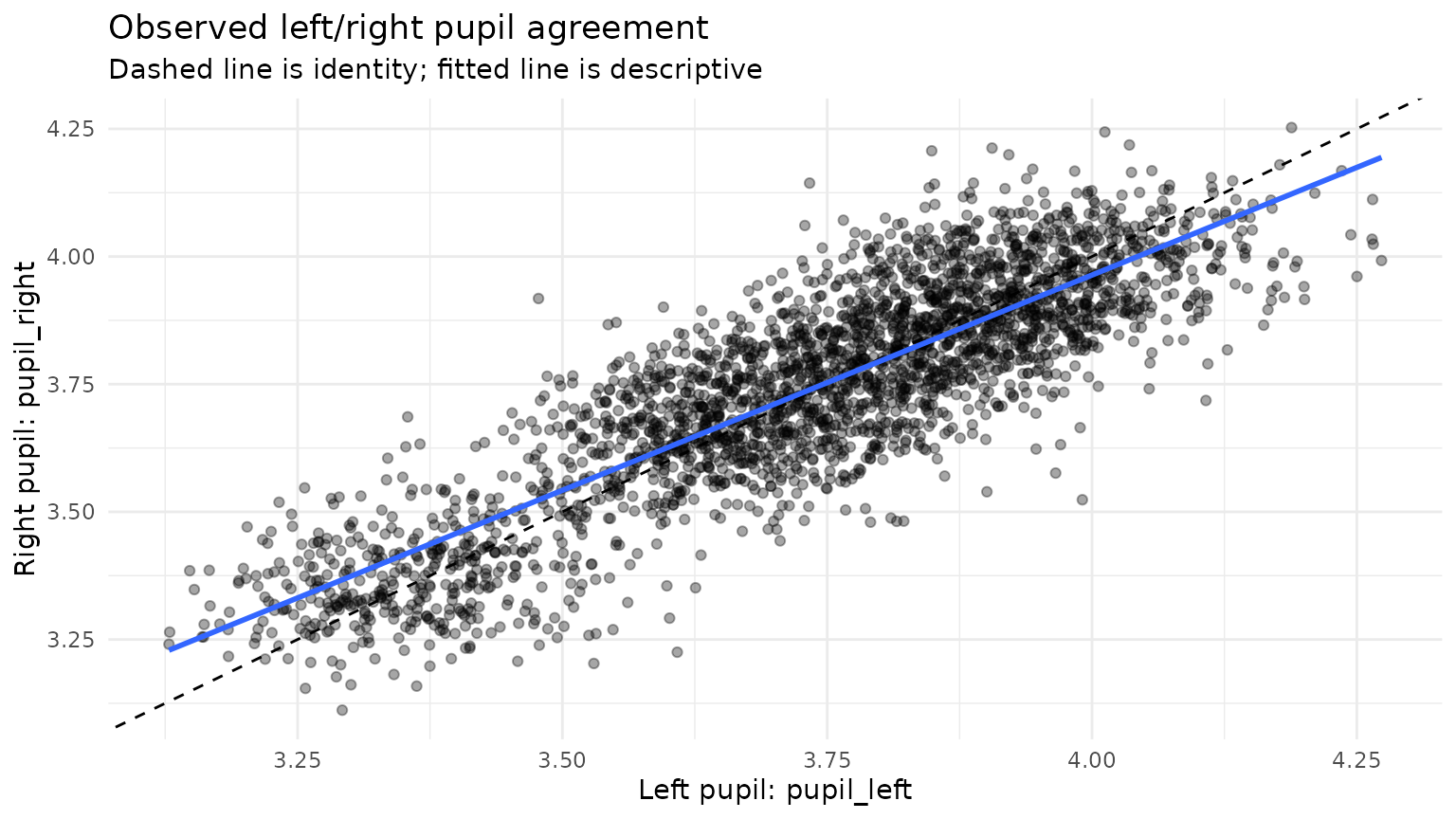
Observed left/right pupil agreement. The dashed identity line is distinct from the fitted descriptive relationship.

plot_gazepoint_binocular_diagnostics(
  pupil,
  type = "bland_altman",
  left_col = "pupil_left",
  right_col = "pupil_right"
)

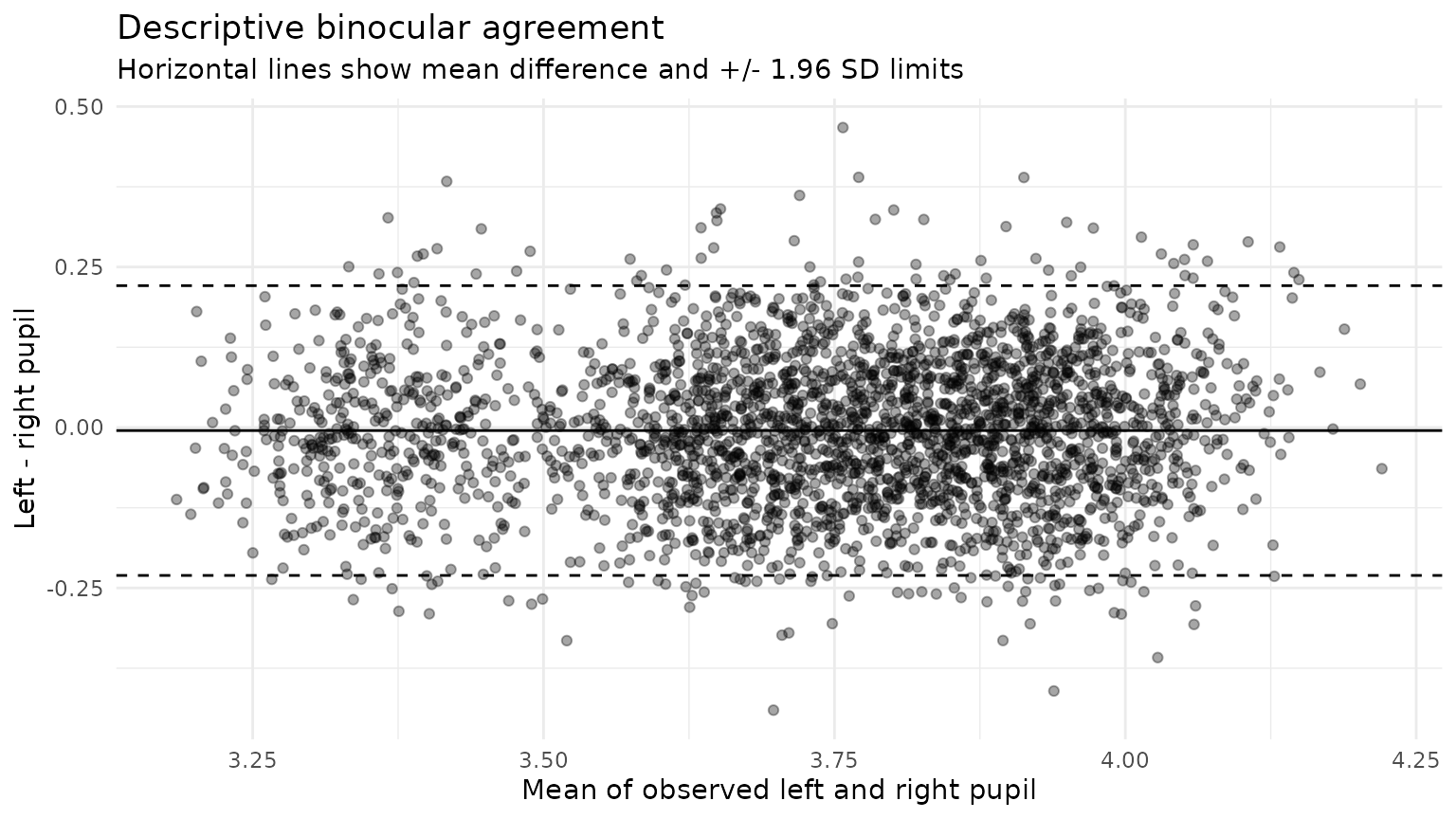
Descriptive left-minus-right agreement across the observed pupil range.

The difference plot is descriptive. Its mean difference and +/-1.96 SD lines should not be interpreted as proof that the two eye channels are interchangeable.

2. Fit auditable bidirectional calibration

The calibration stage fits separate left-from-right and right-from-left models. Here the primary models are participant-specific and a pooled fallback is retained. Fallback is explicit in the returned model table.

calibration <- fit_gazepoint_binocular_calibration(
  pupil,
  left_col = "pupil_left",
  right_col = "pupil_right",
  group_cols = "subject",
  # Default fallback is pooled when primary groups are supplied.
  min_pairs = 80,
  min_unique = 10,
  min_r2 = NULL,
  valid_min = 1,
  valid_max = 9
)

calibration$models[c(
  "model_id", "direction", "calibration_level", "n_pairs",
  "intercept", "slope", "r_squared", "rmse", "mae",
  "eligible", "reason"
)]
#> # A tibble: 14 × 11
#>    model_id direction calibration_level n_pairs intercept slope r_squared   rmse
#>    <chr>    <chr>     <chr>               <int>     <dbl> <dbl>     <dbl>  <dbl>
#>  1 binoc_0… left_fro… subject               459     2.20  0.346    0.118  0.0931
#>  2 binoc_0… right_fr… subject               459     2.24  0.340    0.118  0.0923
#>  3 binoc_0… left_fro… subject               455     2.41  0.343    0.116  0.0919
#>  4 binoc_0… right_fr… subject               455     2.44  0.340    0.116  0.0914
#>  5 binoc_0… left_fro… subject               462     2.53  0.334    0.124  0.0885
#>  6 binoc_0… right_fr… subject               462     2.40  0.370    0.124  0.0931
#>  7 binoc_0… left_fro… subject               466     2.84  0.286    0.0713 0.0985
#>  8 binoc_0… right_fr… subject               466     2.97  0.249    0.0713 0.0920
#>  9 binoc_0… left_fro… subject               454     2.81  0.281    0.0771 0.0916
#> 10 binoc_0… right_fr… subject               454     2.85  0.274    0.0771 0.0904
#> 11 binoc_0… left_fro… subject               463     2.67  0.275    0.0728 0.0967
#> 12 binoc_0… right_fr… subject               463     2.71  0.265    0.0728 0.0949
#> 13 binoc_0… left_fro… pooled               2759     0.454 0.877    0.740  0.112 
#> 14 binoc_0… right_fr… pooled               2759     0.591 0.843    0.740  0.110 
#> # ℹ 3 more variables: mae <dbl>, eligible <lgl>, reason <chr>

min_r2 = NULL is intentional. R-squared is reported, but no universal R-squared threshold is presented as a validity rule. A study can declare a threshold if it has a substantive reason to do so.

3. Validate by hiding values that are actually known

Bilateral observations provide an unusually useful validation opportunity: one eye can be deliberately hidden and reconstructed from the other while its true observed value is retained outside the training data for error calculation.

validation <- validate_gazepoint_binocular_reconstruction(
  pupil,
  left_col = "pupil_left",
  right_col = "pupil_right",
  time_col = "timestamp_ms",
  group_cols = "subject",
  gap_group_cols = c("subject", "trial"),
  direction = "both",
  mask_prop = 0.10,
  mask_mode = "contiguous",
  block_size = 5,
  repeats = 3,
  seed = 1729,
  min_pairs = 80,
  valid_min = 1,
  valid_max = 9
)

validation$summary
#> # A tibble: 2 × 11
#>   direction       repeats total_requested total_predicted prediction_rate   rmse
#>   <chr>             <int>           <int>           <int>           <dbl>  <dbl>
#> 1 left_from_right       3             422             422           1     0.0914
#> 2 right_from_left       3             412             410           0.995 0.0930
#> # ℹ 5 more variables: mae <dbl>, bias <dbl>, median_error <dbl>,
#> #   error_mad <dbl>, correlation <dbl>

The result reports the fraction of requested held-out samples that could actually be reconstructed, together with RMSE, MAE, bias, and correlation.

plot_gazepoint_binocular_diagnostics(validation, type = "validation")
#> Warning: Removed 2 rows containing missing values or values outside the scale range
#> (`geom_point()`).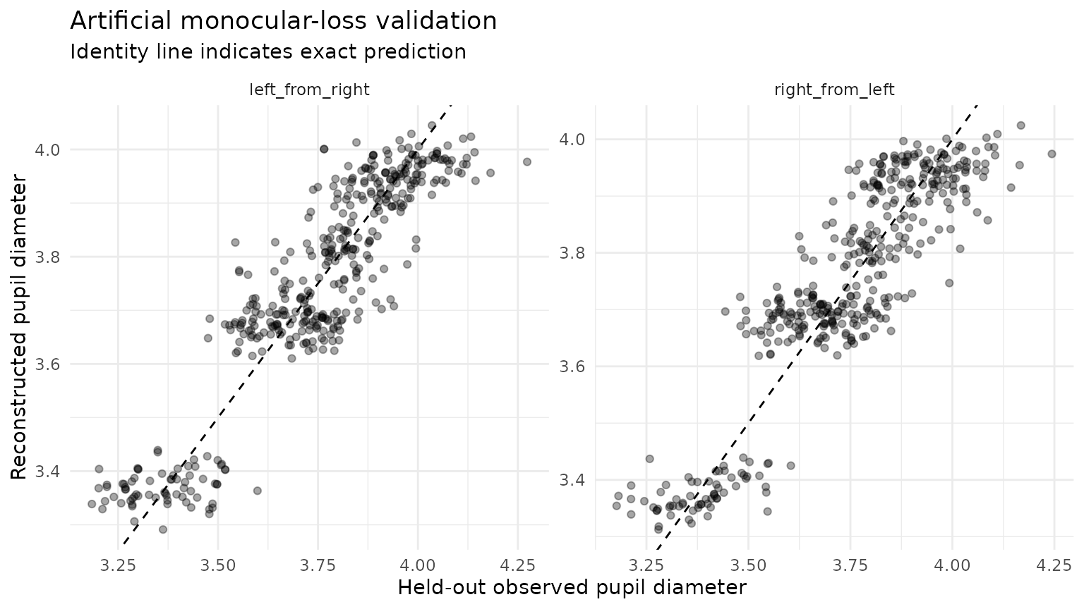

Observed versus reconstructed pupil values under artificial monocular loss.

plot_gazepoint_binocular_diagnostics(validation, type = "residuals")
#> Warning: Removed 2 rows containing missing values or values outside the scale range
#> (`geom_point()`).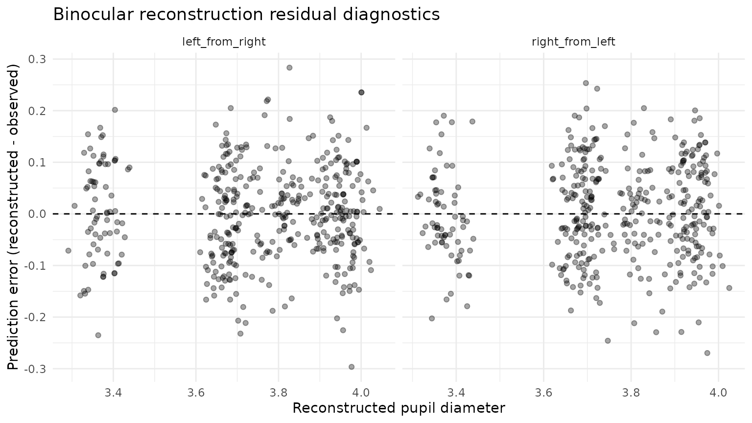

Prediction error as a function of reconstructed pupil diameter.

A good artificial-missingness result is evidence that the declared model predicts held-out bilateral samples well. It cannot show that naturally missing samples follow the same missingness process.

4. Reconstruct under explicit gates

The following policy allows regression reconstruction only for missing-eye runs no longer than 150 ms, disallows predictor extrapolation, and excludes any row that is already marked as a blink.

reconstructed <- reconstruct_gazepoint_binocular_pupil(
  pupil,
  left_col = "pupil_left",
  right_col = "pupil_right",
  time_col = "timestamp_ms",
  group_cols = "subject",
  gap_group_cols = c("subject", "trial"),
  method = "linear_regression",
  calibration = calibration,
  time_unit = "milliseconds",
  max_gap_ms = 150,
  allow_edge_gaps = TRUE,
  allow_extrapolation = FALSE,
  valid_min = 1,
  valid_max = 9,
  exclude_flag_cols = "blink"
)

table(reconstructed$gp3_binocular_status)
#> 
#>  bilateral_observed    both_unavailable  left_reconstructed right_reconstructed 
#>                2759                  78                  23                  20

The original columns are untouched. The added columns distinguish the observed and final channels, prediction direction, model identity, calibration level, model R-squared, extrapolation status, gap duration, and row-level outcome.

reconstructed[75:90, c(
  "pupil_left", "pupil_right",
  "gp3_binocular_left_observed", "gp3_binocular_right_observed",
  "gp3_binocular_left_final", "gp3_binocular_right_final",
  "gp3_binocular_reconstructed", "gp3_binocular_model_id",
  "gp3_binocular_gap_ms", "gp3_binocular_status"
)]
#>    pupil_left pupil_right gp3_binocular_left_observed
#> 75   3.313574    3.300916                    3.313574
#> 76   3.365124    3.324580                    3.365124
#> 77   3.398240    3.340684                    3.398240
#> 78   3.529691    3.203018                    3.529691
#> 79   3.225775    3.263195                    3.225775
#> 80         NA    3.261327                          NA
#> 81         NA    3.197705                          NA
#> 82         NA    3.289575                          NA
#> 83         NA    3.392627                          NA
#> 84         NA    3.430466                          NA
#> 85   3.531753    3.261433                    3.531753
#> 86   3.167372    3.315744                    3.167372
#> 87   3.321451    3.323391                    3.321451
#> 88   3.241113    3.212430                    3.241113
#> 89   3.395153    3.212441                    3.395153
#> 90   3.286586    3.176851                    3.286586
#>    gp3_binocular_right_observed gp3_binocular_left_final
#> 75                     3.300916                 3.313574
#> 76                     3.324580                 3.365124
#> 77                     3.340684                 3.398240
#> 78                     3.203018                 3.529691
#> 79                     3.263195                 3.225775
#> 80                     3.261327                 3.330176
#> 81                     3.197705                 3.308135
#> 82                     3.289575                 3.339962
#> 83                     3.392627                 3.375662
#> 84                     3.430466                 3.388771
#> 85                     3.261433                 3.531753
#> 86                     3.315744                 3.167372
#> 87                     3.323391                 3.321451
#> 88                     3.212430                 3.241113
#> 89                     3.212441                 3.395153
#> 90                     3.176851                 3.286586
#>    gp3_binocular_right_final gp3_binocular_reconstructed
#> 75                  3.300916                       FALSE
#> 76                  3.324580                       FALSE
#> 77                  3.340684                       FALSE
#> 78                  3.203018                       FALSE
#> 79                  3.263195                       FALSE
#> 80                  3.261327                        TRUE
#> 81                  3.197705                        TRUE
#> 82                  3.289575                        TRUE
#> 83                  3.392627                        TRUE
#> 84                  3.430466                        TRUE
#> 85                  3.261433                       FALSE
#> 86                  3.315744                       FALSE
#> 87                  3.323391                       FALSE
#> 88                  3.212430                       FALSE
#> 89                  3.212441                       FALSE
#> 90                  3.176851                       FALSE
#>       gp3_binocular_model_id gp3_binocular_gap_ms gp3_binocular_status
#> 75                      <NA>                   NA   bilateral_observed
#> 76                      <NA>                   NA   bilateral_observed
#> 77                      <NA>                   NA   bilateral_observed
#> 78                      <NA>                   NA   bilateral_observed
#> 79                      <NA>                   NA   bilateral_observed
#> 80 binoc_001_left_from_right                83.35   left_reconstructed
#> 81 binoc_001_left_from_right                83.35   left_reconstructed
#> 82 binoc_001_left_from_right                83.35   left_reconstructed
#> 83 binoc_001_left_from_right                83.35   left_reconstructed
#> 84 binoc_001_left_from_right                83.35   left_reconstructed
#> 85                      <NA>                   NA   bilateral_observed
#> 86                      <NA>                   NA   bilateral_observed
#> 87                      <NA>                   NA   bilateral_observed
#> 88                      <NA>                   NA   bilateral_observed
#> 89                      <NA>                   NA   bilateral_observed
#> 90                      <NA>                   NA   bilateral_observed

5. Construct a combined signal as a separate decision

Reconstruction does not silently create the outcome variable. The analyst chooses how a combined pupil signal should be constructed.

combined <- construct_gazepoint_combined_pupil(
  reconstructed,
  left_col = "pupil_left",
  right_col = "pupil_right",
  policy = "reconstructed_mean",
  output_col = "pupil_reconstruction_policy",
  status_col = "pupil_reconstruction_source"
)

table(combined$pupil_reconstruction_source)
#> 
#>            bilateral_observed bilateral_with_reconstruction 
#>                          2759                            43 
#>                   unavailable 
#>                            78

Alternative policies include complete_case, available_eye, left_only, and right_only.

6. Inspect temporal provenance

plot_gazepoint_binocular_diagnostics(reconstructed, type = "trace")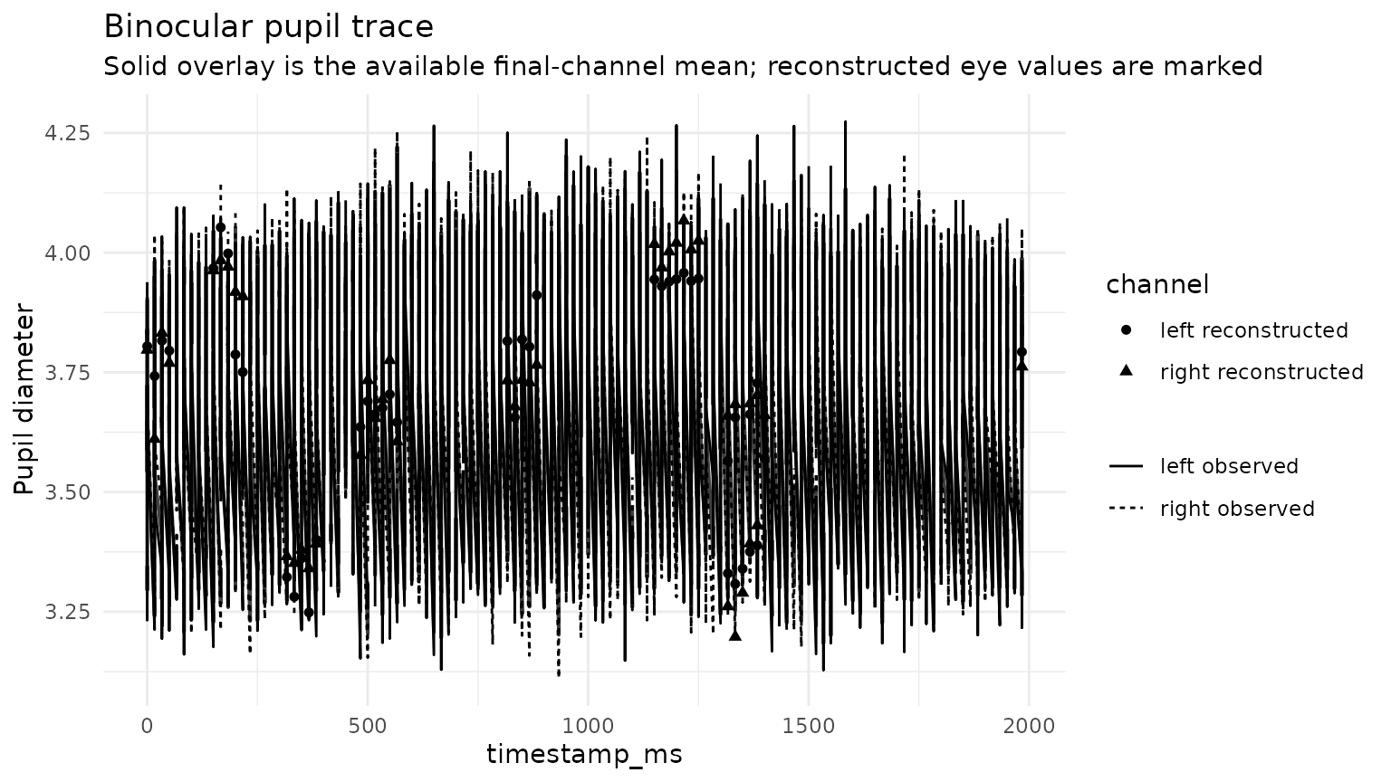

Observed binocular traces with reconstructed final values marked explicitly.

plot_gazepoint_binocular_diagnostics(reconstructed, type = "timeline")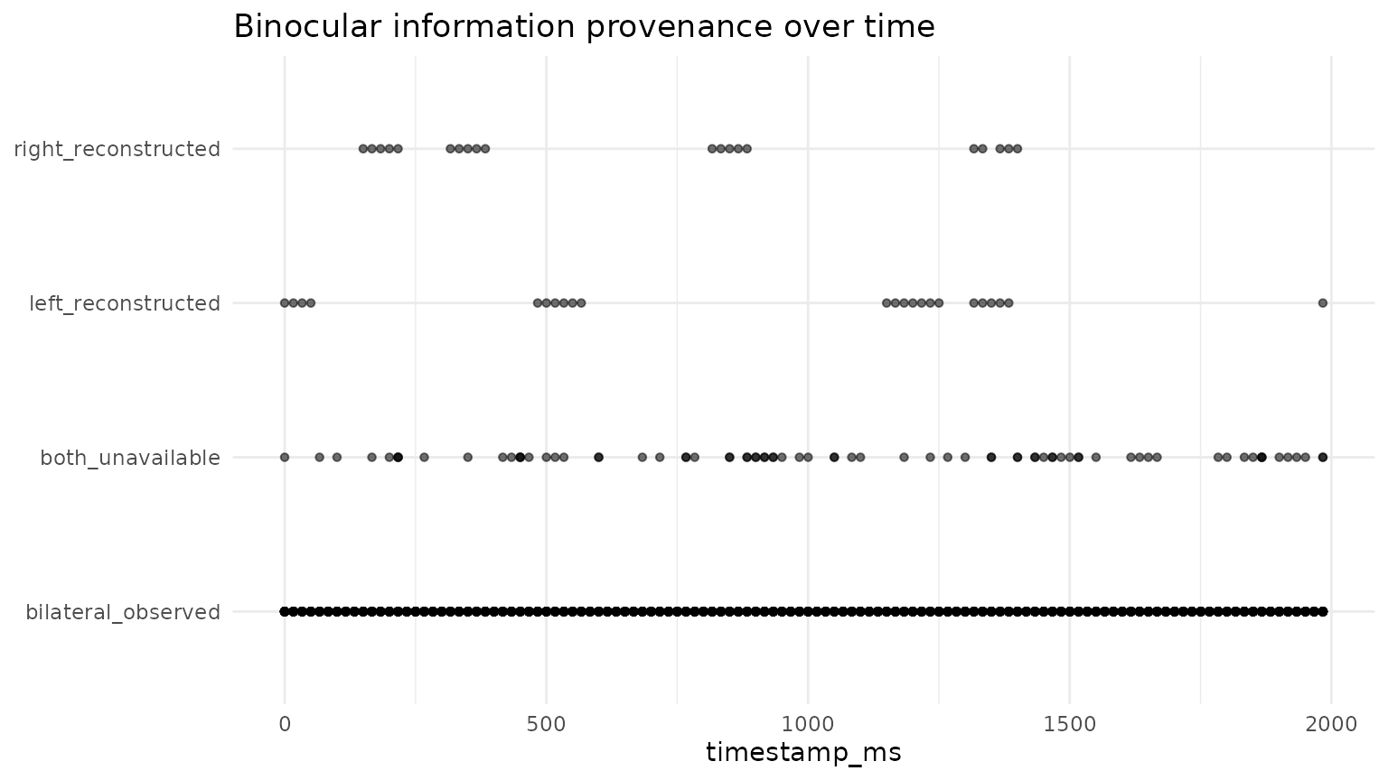

Row-level binocular information status over time.

plot_gazepoint_binocular_diagnostics(reconstructed, type = "gaps", bins = 15)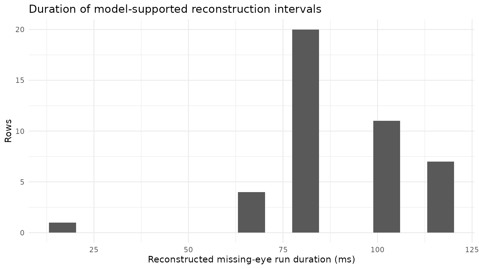

Duration of missing-eye runs that were reconstructed.

The dashboard option returns a list of these ggplot objects rather than adding a layout dependency.

dashboard <- plot_gazepoint_binocular_diagnostics(
  reconstructed,
  type = "dashboard"
)
names(dashboard)
#> [1] "trace"     "agreement" "timeline"  "gaps"

7. Audit reconstruction burden and condition imbalance

audit <- audit_gazepoint_binocular_reconstruction(
  reconstructed,
  by = "condition",
  max_reconstruction_prop = 0.20,
  max_group_rate_difference = 0.10
)

audit$overall
#> # A tibble: 1 × 11
#>   group_key      n n_bilateral_observed n_reconstructed n_monocular_unreconstr…¹
#>   <chr>      <int>                <int>           <int>                    <int>
#> 1 __pooled__  2880                 2759              43                        0
#> # ℹ abbreviated name: ¹n_monocular_unreconstructed
#> # ℹ 6 more variables: n_unavailable <int>, n_blocked <int>,
#> #   bilateral_observed_fraction <dbl>, reconstruction_fraction <dbl>,
#> #   monocular_unreconstructed_fraction <dbl>, unavailable_fraction <dbl>
audit$by_group
#> # A tibble: 2 × 12
#>   condition group_key               n n_bilateral_observed n_reconstructed
#>   <chr>     <chr>               <int>                <int>           <int>
#> 1 control   condition=control    1440                 1369              27
#> 2 treatment condition=treatment  1440                 1390              16
#> # ℹ 7 more variables: n_monocular_unreconstructed <int>, n_unavailable <int>,
#> #   n_blocked <int>, bilateral_observed_fraction <dbl>,
#> #   reconstruction_fraction <dbl>, monocular_unreconstructed_fraction <dbl>,
#> #   unavailable_fraction <dbl>
audit$reconstruction_shift
#> # A tibble: 1 × 5
#>   n_reconstructed_rows_with_shift mean_reconstruction_s…¹ median_reconstructio…²
#>                             <int>                   <dbl>                  <dbl>
#> 1                              43                0.000772               -0.00234
#> # ℹ abbreviated names: ¹mean_reconstruction_shift, ²median_reconstruction_shift
#> # ℹ 2 more variables: mean_absolute_reconstruction_shift <dbl>,
#> #   max_absolute_reconstruction_shift <dbl>
audit$audit
#> # A tibble: 1 × 5
#>   status reconstruction_fraction reconstruction_threshold burden_flag
#>   <chr>                    <dbl>                    <dbl> <lgl>      
#> 1 ok                      0.0149                      0.2 FALSE      
#> # ℹ 1 more variable: imbalance_flag <lgl>

The thresholds above are governance flags. They are not universal statistical or physiological validity cutoffs.

plot_gazepoint_binocular_diagnostics(audit, type = "burden")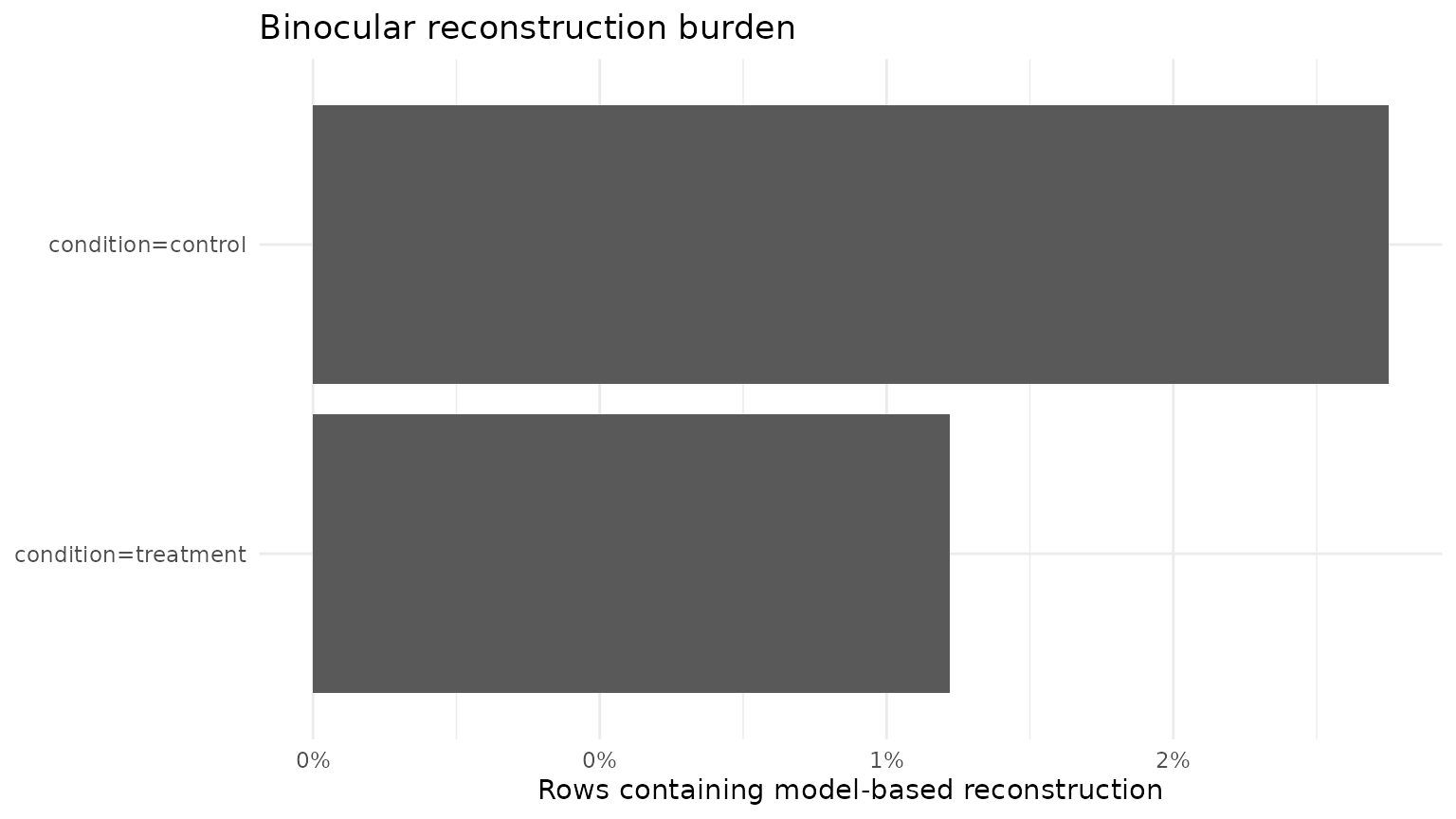

Reconstruction burden by experimental condition.

8. Compare alternative pupil-construction policies

sensitivity <- analyse_gazepoint_binocular_sensitivity(
  reconstructed,
  left_col = "pupil_left",
  right_col = "pupil_right",
  policies = c(
    "complete_case",
    "available_eye",
    "reconstructed_mean",
    "left_only",
    "right_only"
  ),
  condition_col = "condition"
)

sensitivity$summary
#> # A tibble: 5 × 9
#>   policy    group_key n_total n_usable missing_fraction  mean    sd median   mad
#>   <chr>     <chr>       <int>    <int>            <dbl> <dbl> <dbl>  <dbl> <dbl>
#> 1 complete… __pooled…    2880     2759           0.0420  3.74 0.210   3.77 0.138
#> 2 availabl… __pooled…    2880     2802           0.0271  3.74 0.211   3.77 0.138
#> 3 reconstr… __pooled…    2880     2802           0.0271  3.74 0.210   3.77 0.138
#> 4 left_only __pooled…    2880     2779           0.0351  3.74 0.220   3.77 0.145
#> 5 right_on… __pooled…    2880     2782           0.0340  3.74 0.216   3.77 0.140
sensitivity$correlations
#> # A tibble: 10 × 6
#>    policy_1           policy_2           n_complete correlation mean_difference
#>    <chr>              <chr>                   <int>       <dbl>           <dbl>
#>  1 complete_case      available_eye            2759       1           0        
#>  2 complete_case      reconstructed_mean       2759       1           0        
#>  3 complete_case      left_only                2759       0.965       0.00237  
#>  4 complete_case      right_only               2759       0.964      -0.00237  
#>  5 available_eye      reconstructed_mean       2802       1.000      -0.0000119
#>  6 available_eye      left_only                2779       0.965       0.00236  
#>  7 available_eye      right_only               2782       0.964      -0.00235  
#>  8 reconstructed_mean left_only                2779       0.965       0.00240  
#>  9 reconstructed_mean right_only               2782       0.964      -0.00239  
#> 10 left_only          right_only               2759       0.860      -0.00475  
#> # ℹ 1 more variable: mean_absolute_difference <dbl>
sensitivity$condition_contrasts
#> # A tibble: 5 × 4
#>   policy             reference comparison mean_difference
#>   <chr>              <chr>     <chr>                <dbl>
#> 1 complete_case      control   treatment           0.0880
#> 2 available_eye      control   treatment           0.0913
#> 3 reconstructed_mean control   treatment           0.0908
#> 4 left_only          control   treatment           0.0874
#> 5 right_only         control   treatment           0.0918

The condition contrasts are descriptive mean differences only. The function deliberately does not generate a new p-value for every preprocessing policy.

plot_gazepoint_binocular_diagnostics(sensitivity, type = "sensitivity")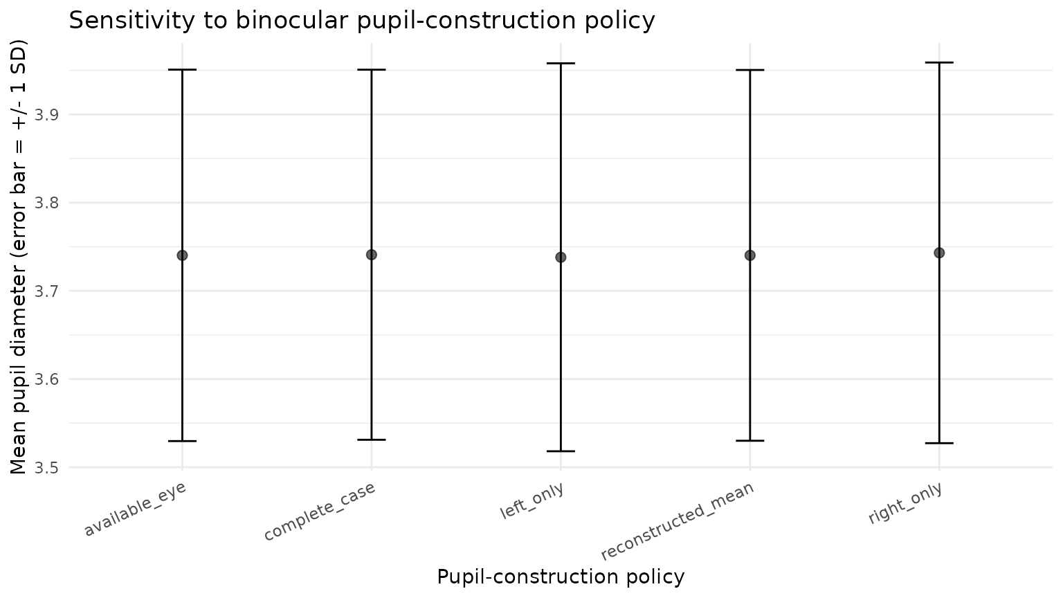

Mean pupil diameter under alternative binocular construction policies.

9. Reconstruction and PCHIP are different decisions

Ong et al. (2025) used PCHIP to create a common high-frequency time base, removed interpolated segments corresponding to original gaps longer than 250 ms, and then used cross-eye regression when one eye remained unavailable. gp3tools does not hard-code that study-specific sequence or cutoff.

For a workflow that uses cross-eye reconstruction first, PCHIP can be applied afterwards to remaining short gaps in the explicitly constructed signal. This is useful when the analyst wants to keep model-based cross-eye support separate from temporal interpolation.

if (requireNamespace("pracma", quietly = TRUE)) {
  pchip <- interpolate_gazepoint_pupil_pchip(
    combined,
    pupil_col = "pupil_reconstruction_policy",
    time_col = "timestamp_ms",
    grouping_cols = c("subject", "trial"),
    max_gap_ms = 150,
    output_col = "pupil_after_reconstruction_pchip",
    flag_col = "pupil_pchip_after_reconstruction",
    status_col = "pupil_pchip_status"
  )

  table(pchip$pupil_pchip_after_reconstruction)
}
#> 
#> FALSE  TRUE 
#>  2805    75

A study can reverse the order if its measurement and synchronization design requires it, but it should report the choice. The two operations should not be collapsed into an undocumented generic “imputation” step.

10. Baseline correction follows the declared combined signal

After choosing the pupil-construction policy, the resulting signal can enter the existing baseline and smoothing workflow. Baseline windows should be designed prospectively when possible. Ong et al. selected the first period with at least 400 ms of consecutive valid bilateral data because a controlled baseline had not been collected; the authors identify this as a limitation rather than a universal rule.

A study with an experimental baseline can use the existing baseline_correct_gazepoint_pupil() interface on the declared combined column.

baseline_corrected <- baseline_correct_gazepoint_pupil(
  combined,
  pupil_col = "pupil_reconstruction_policy",
  time_col = "timestamp_ms",
  group_cols = c("subject", "trial"),
  baseline_window = c(0, 200),
  min_baseline_samples = 5
)

The example is not executed because the synthetic trials are not designed as a real baseline experiment; the code illustrates where the existing function belongs in the workflow.

11. Manuscript-ready reporting

reporting <- summarise_gazepoint_binocular_reporting(
  reconstructed,
  audit = audit,
  validation = validation
)

reporting$summary
#> # A tibble: 1 × 9
#>   n_rows n_reconstructed reconstruction_fraction bilateral_observed_fraction
#>    <int>           <int>                   <dbl>                       <dbl>
#> 1   2880              43                  0.0149                       0.958
#> # ℹ 5 more variables: monocular_unreconstructed_fraction <dbl>,
#> #   audit_status <chr>, method <chr>, max_gap_ms <dbl>,
#> #   allow_extrapolation <lgl>
cat(reporting$text)
#> Binocular pupil handling used the declared `linear_regression` policy. Of 2880 rows, 43 (1.5%) contained model-based cross-eye reconstruction; 95.8% were retained as directly observed bilateral samples and 0.0% remained monocular without reconstruction. Eligible cross-eye calibration models used a median of 462 paired observations; the median in-sample R-squared was 0.116. Artificial monocular-loss validation reconstructed 99.8% of requested held-out values, with RMSE 0.092 and MAE 0.075. Reconstructed values were retained as predicted values with explicit row-level provenance; they were not treated as independently measured pupil observations.

The returned limitations can be reused when preparing a methods supplement or analysis decision log.

reporting$limitations
#> [1] "Cross-eye prediction is a preprocessing reconstruction and does not recover an independently observed biological truth."                                            
#> [2] "Artificial masking quantifies prediction performance on observed bilateral samples but cannot establish the missingness mechanism of naturally unavailable samples."
#> [3] "Calibration diagnostics and reconstruction burden should be reported alongside downstream sensitivity analyses."                                                    
#> [4] "Temporal interpolation and cross-eye reconstruction should remain separately declared analytical decisions."

12. When reconstruction should not be used

A conservative workflow should retain an explicit reconstruction_ineligible or reconstruction_blocked_* status when:

too few bilateral observations are available for calibration;
one eye has effectively no variance;
the fitted relationship is unstable or biologically implausible;
a prediction requires prohibited extrapolation;
the predicted diameter violates declared bounds;
the missing-eye run exceeds the declared duration limit;
a row is explicitly excluded because it is blink/artifact contaminated;
pseudo-missing validation shows unacceptable prediction error for the intended use;
reconstruction burden is so large or imbalanced that the downstream result is materially policy-dependent.

The framework therefore permits a scientifically meaningful outcome of no reconstruction.

13. Relationship to the existing lightweight binocular helpers

Use combine_gazepoint_eyes() when a transparent sample-wise fusion rule is all that is required. Use the existing regress_gazepoint_pupils() workflow when its documented regression-fusion behavior matches the analysis plan. Use the functions in this article when the goal is specifically to reconstruct a temporarily missing eye with explicit calibration eligibility, gap/extrapolation gates, pseudo-missing validation, row-level provenance, reconstruction burden, and sensitivity analysis.

No existing function changes its default behavior.

References

Ong, J., He, W., Maglanque, P., Jiang, X., Gillman, L. M., Vergis, A., & Hardy, K. (2025). A Preprocessing Pipeline for Pupillometry Signal from Multimodal iMotion Data. Sensors, 25(15), 4737. doi:10.3390/s25154737.