AOI Labelling, Sliding Windows, and Fixation Simulation
Source:vignettes/articles/aoi-window-feature-engineering.Rmd
aoi-window-feature-engineering.RmdPurpose
This article combines three reusable feature-engineering helpers:
- simulate Gazepoint-like fixation events;
- add rectangular AOI membership to sample-level coordinates;
- summarise gaze and pupil measures in sliding time windows.
Simulate fixation events
fixations <- simulate_gazepoint_fixations(
  n_subjects = 4,
  n_fix = 30,
  coordinate_system = "pixels",
  screen_width = 1280,
  screen_height = 720,
  sd = 45,
  seed = 2026
)

fixations
#> # A tibble: 120 × 17
#>    USER_ID MEDIA_ID    FPOGID FPOGS  FPOGD FPOGX FPOGY FPOGV subject fixation_id
#>    <chr>   <chr>        <int> <dbl>  <dbl> <dbl> <dbl> <int> <chr>         <int>
#>  1 P001    simulated_…      1 0     0.292  0.593 0.483     1 P001              1
#>  2 P001    simulated_…      2 0.327 0.164  0.577 0.532     1 P001              2
#>  3 P001    simulated_…      3 0.503 0.261  0.520 0.543     1 P001              3
#>  4 P001    simulated_…      4 0.816 0.243  0.482 0.640     1 P001              4
#>  5 P001    simulated_…      5 1.16  0.197  0.509 0.644     1 P001              5
#>  6 P001    simulated_…      6 1.36  0.0487 0.470 0.606     1 P001              6
#>  7 P001    simulated_…      7 1.46  0.191  0.496 0.627     1 P001              7
#>  8 P001    simulated_…      8 1.66  0.168  0.442 0.587     1 P001              8
#>  9 P001    simulated_…      9 1.83  0.259  0.438 0.520     1 P001              9
#> 10 P001    simulated_…     10 2.11  0.212  0.430 0.506     1 P001             10
#> # ℹ 110 more rows
#> # ℹ 7 more variables: start_time <dbl>, end_time <dbl>, duration <dbl>,
#> #   duration_ms <dbl>, x <dbl>, y <dbl>, coordinate_system <chr>
ggplot(fixations, aes(x, y, group = USER_ID)) +
  geom_path(alpha = 0.5) +
  geom_point(aes(size = duration_ms), alpha = 0.7) +
  scale_y_reverse() +
  facet_wrap(~ USER_ID) +
  coord_fixed() +
  labs(
    x = "Screen x (pixels)",
    y = "Screen y (pixels)",
    size = "Duration (ms)",
    title = "Simulated fixation paths"
  ) +
  theme_minimal()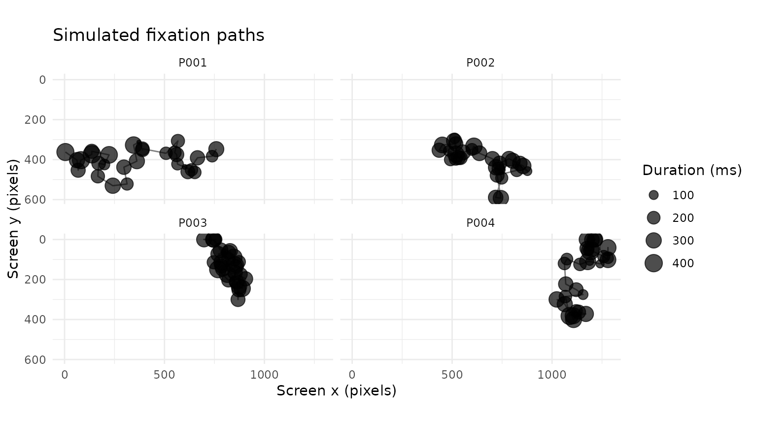
Create a sample-level trace
set.seed(2026)

n <- 500
samples <- data.frame(
  USER_ID = rep(c("P01", "P02"), each = n / 2),
  trial = rep(c("T01", "T02"), each = n / 2),
  TIME = rep(seq(0, 2.49, by = 0.01), 2),
  FPOGX = c(
    seq(0.15, 0.85, length.out = n / 2),
    seq(0.85, 0.15, length.out = n / 2)
  ) + rnorm(n, 0, 0.015),
  FPOGY = 0.50 + rnorm(n, 0, 0.06),
  mean_pupil = 3.3 + rnorm(n, 0, 0.05)
)

aoi_defs <- data.frame(
  name = c("left", "right"),
  L = c(0.00, 0.55),
  R = c(0.45, 1.00),
  T = c(0.20, 0.20),
  B = c(0.80, 0.80)
)
Add AOI membership
labelled <- add_gazepoint_aoi(
  samples,
  aoi_defs,
  output = "both",
  overlap = "error"
)

table(labelled$aoi_current, useNA = "ifany")
#>
#>    left outside   right
#>     217      70     213
ggplot(labelled, aes(FPOGX, FPOGY, shape = aoi_current)) +
  geom_point(alpha = 0.45) +
  scale_y_reverse() +
  facet_wrap(~ USER_ID) +
  coord_fixed() +
  labs(
    x = "Normalized x",
    y = "Normalized y",
    shape = "AOI",
    title = "Rectangular AOI classification"
  ) +
  theme_minimal()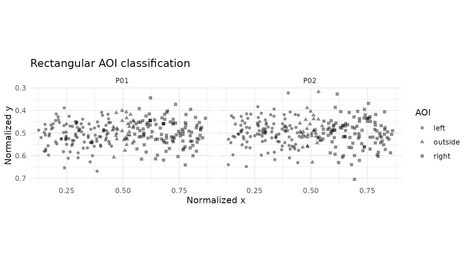
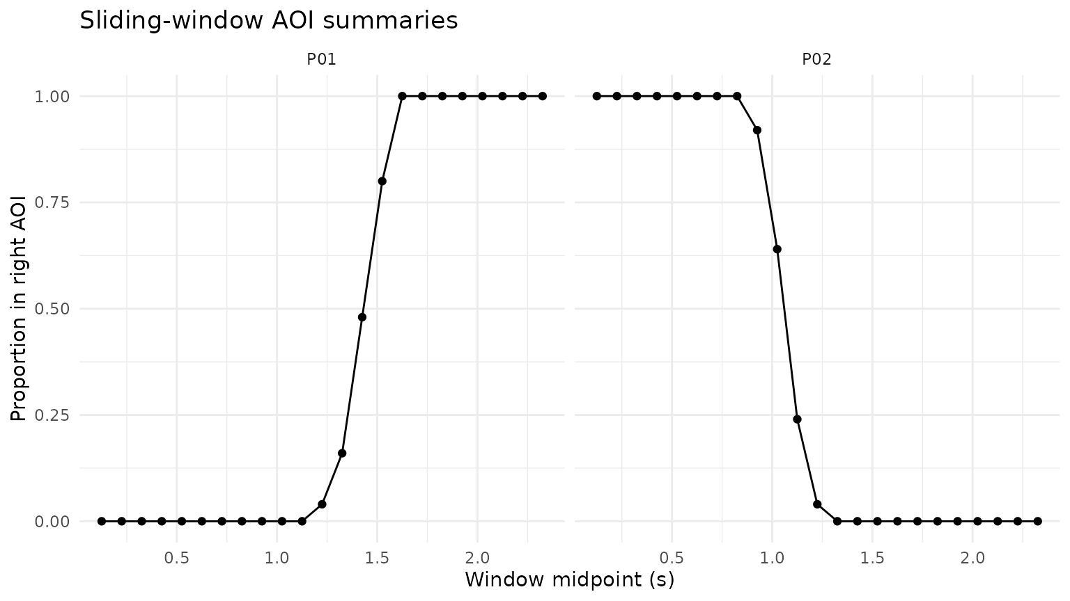
Sliding-window summaries
labelled$right_aoi_numeric <- as.numeric(labelled$aoi_right)

windows <- analyze_gazepoint_window(
  labelled,
  window_size = 250,
  step = 100,
  summary_stats = c("mean", "sd", "valid_prop"),
  by = c("USER_ID", "trial"),
  value_cols = c("mean_pupil", "right_aoi_numeric")
)

windows
#> # A tibble: 46 × 15
#>    USER_ID trial window_start window_end window_mid window_size window_step
#>    <chr>   <chr>        <dbl>      <dbl>      <dbl>       <dbl>       <dbl>
#>  1 P01     T01            0         0.25      0.125         250         100
#>  2 P01     T01            0.1       0.35      0.225         250         100
#>  3 P01     T01            0.2       0.45      0.325         250         100
#>  4 P01     T01            0.3       0.55      0.425         250         100
#>  5 P01     T01            0.4       0.65      0.525         250         100
#>  6 P01     T01            0.5       0.75      0.625         250         100
#>  7 P01     T01            0.6       0.85      0.725         250         100
#>  8 P01     T01            0.7       0.95      0.825         250         100
#>  9 P01     T01            0.8       1.05      0.925         250         100
#> 10 P01     T01            0.9       1.15      1.02          250         100
#> # ℹ 36 more rows
#> # ℹ 8 more variables: window_unit <chr>, n_samples <int>,
#> #   mean_pupil_mean <dbl>, mean_pupil_sd <dbl>, mean_pupil_valid_prop <dbl>,
#> #   right_aoi_numeric_mean <dbl>, right_aoi_numeric_sd <dbl>,
#> #   right_aoi_numeric_valid_prop <dbl>
ggplot(
  windows,
  aes(window_mid, right_aoi_numeric_mean, group = USER_ID)
) +
  geom_line() +
  geom_point() +
  facet_wrap(~ USER_ID) +
  labs(
    x = "Window midpoint (s)",
    y = "Proportion in right AOI",
    title = "Sliding-window AOI summaries"
  ) +
  theme_minimal()