Scanpath and quality-control quick wins
Source:vignettes/articles/scanpath-qc-quick-wins.Rmd
scanpath-qc-quick-wins.RmdThis article demonstrates a compact set of descriptive helpers for privacy-safe examples, binocular pupil preparation, trackloss review, time-series plotting, and multi-scanpath visual inspection. These helpers are intended for transparent quality control and documentation. They do not replace study-specific preprocessing decisions or inferential modelling.
Simulate pupil and gaze data
simulate_gazepoint_pupil_data() creates a small
synthetic data set with participant, trial, condition, time-bin,
gaze-coordinate, left-pupil, right-pupil, blink, trackloss, and
combined-pupil columns.
synthetic <- simulate_gazepoint_pupil_data(
  n_subjects = 4,
  n_trials = 4,
  n_time_bins = 20,
  conditions = c("control", "treatment"),
  blink_probability = 0.05,
  seed = 123
)

head(synthetic)
#>   subject trial condition time_bin timestamp_ms    gaze_x   gaze_y pupil_left
#> 1    S001     1   control        1         0.00  993.1529 498.0263   3.355974
#> 2    S001     1   control        2        16.67  977.2926 794.7236   3.484336
#> 3    S001     1   control        3        33.34  950.9250 535.9970   3.385504
#> 4    S001     1   control        4        50.01 1219.3699 504.5001   3.248926
#> 5    S001     1   control        5        66.68  993.1579 563.9892   3.296683
#> 6    S001     1   control        6        83.35  941.0047 414.5260   3.317478
#>   pupil_right blink trackloss    pupil
#> 1    3.303798 FALSE     FALSE 3.329886
#> 2    3.401831 FALSE     FALSE 3.443084
#> 3    3.343765 FALSE     FALSE 3.364635
#> 4    3.400768 FALSE     FALSE 3.324847
#> 5    3.458472 FALSE     FALSE 3.377578
#> 6    3.353714 FALSE     FALSE 3.335596
The generator is designed for examples and tests. It should not be used to make claims about empirical pupil physiology.
Combine left and right pupil channels
combine_gazepoint_eyes() combines two eye-specific
numeric columns into a single analysis column. The default method
averages available left/right values. Other options can prefer one eye
or choose the globally less-missing eye.
combined <- combine_gazepoint_eyes(
  synthetic,
  left_col = "pupil_left",
  right_col = "pupil_right",
  output_col = "pupil_combined",
  method = "mean",
  valid_min = 1,
  valid_max = 9
)

head(combined[, c("pupil_left", "pupil_right", "pupil_combined")])
#>   pupil_left pupil_right pupil_combined
#> 1   3.355974    3.303798       3.329886
#> 2   3.484336    3.401831       3.443084
#> 3   3.385504    3.343765       3.364635
#> 4   3.248926    3.400768       3.324847
#> 5   3.296683    3.458472       3.377578
#> 6   3.317478    3.353714       3.335596
Flag groups by trackloss
clean_gazepoint_by_trackloss() computes trackloss rates
globally or within grouping columns. Here, participant-trial groups with
more than 20% trackloss are flagged.
trackloss_flagged <- clean_gazepoint_by_trackloss(
  synthetic,
  group_cols = c("subject", "trial"),
  tracking_col = "trackloss",
  max_trackloss = 0.20,
  action = "flag"
)

head(trackloss_flagged[, c("subject", "trial", "trackloss", ".gp3_trackloss_rate", ".gp3_trackloss_exclude")])
#>   subject trial trackloss .gp3_trackloss_rate .gp3_trackloss_exclude
#> 1    S001     1     FALSE                0.95                   TRUE
#> 2    S001     1     FALSE                0.95                   TRUE
#> 3    S001     1     FALSE                0.95                   TRUE
#> 4    S001     1     FALSE                0.95                   TRUE
#> 5    S001     1     FALSE                0.95                   TRUE
#> 6    S001     1     FALSE                0.95                   TRUE
A compact group-level summary is stored as an attribute.
head(attr(trackloss_flagged, "gp3_trackloss_summary"))
#>   group_id n_rows n_trackloss_rows trackloss_rate exclude
#> 1   S001.1     20               19           0.95    TRUE
#> 2   S001.2     20               19           0.95    TRUE
#> 3   S001.3     20               19           0.95    TRUE
#> 4   S001.4     20               17           0.85    TRUE
#> 5   S002.1     20               19           0.95    TRUE
#> 6   S002.2     20               20           1.00    TRUE
The same helper can filter high-trackloss groups, but filtering should normally be reported as an explicit preprocessing decision.
Plot a descriptive time series
plot_gazepoint_time_series() provides a general
descriptive line plot for pupil, gaze, AOI, or other time-varying
measures that have already been prepared by the user.
plot_gazepoint_time_series(
  synthetic,
  time_col = "time_bin",
  value_col = "pupil",
  group_cols = c("subject", "trial"),
  colour_col = "condition",
  title = "Synthetic pupil time series",
  x_label = "Time bin",
  y_label = "Pupil size"
)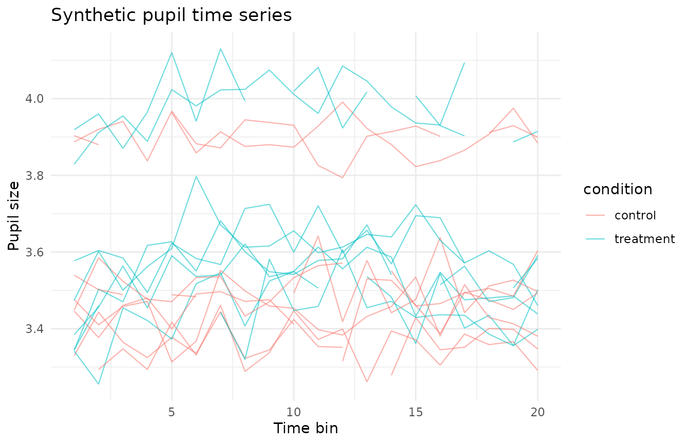
This plot is descriptive. It does not smooth, model, or test condition differences.
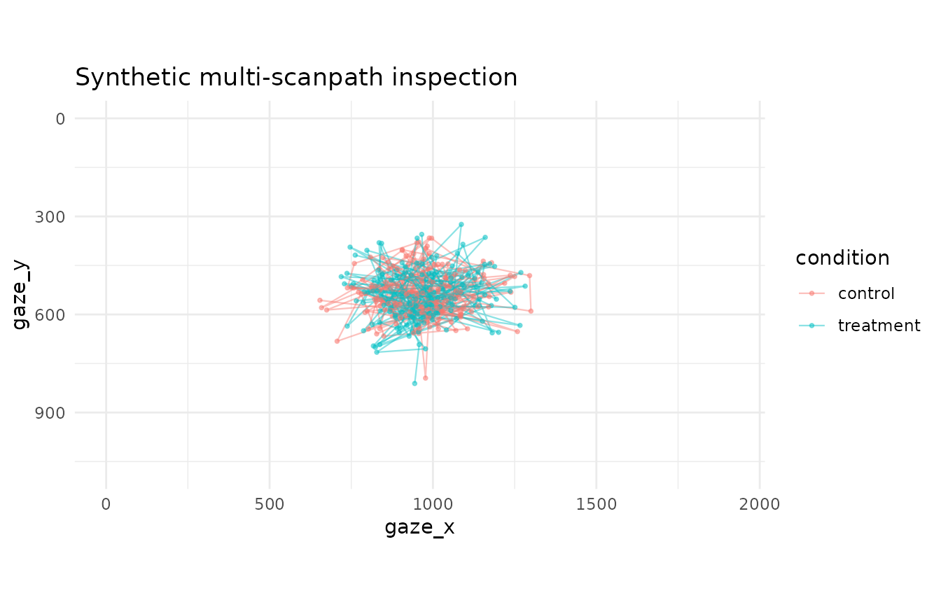
Plot multiple scanpaths
plot_gazepoint_scanpaths() supports quick visual
inspection of gaze paths across participants, trials, or conditions.
plot_gazepoint_scanpaths(
  synthetic,
  x_col = "gaze_x",
  y_col = "gaze_y",
  order_col = "time_bin",
  group_cols = c("subject", "trial"),
  colour_col = "condition",
  screen_width = 1920,
  screen_height = 1080,
  title = "Synthetic multi-scanpath inspection"
)
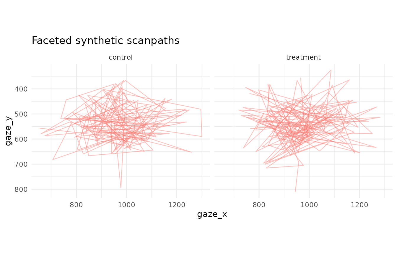
For crowded data, faceting can make trial or condition-level review easier.
plot_gazepoint_scanpaths(
  synthetic,
  x_col = "gaze_x",
  y_col = "gaze_y",
  order_col = "time_bin",
  group_cols = c("subject", "trial"),
  facet_col = "condition",
  show_points = FALSE,
  title = "Faceted synthetic scanpaths"
)
Audit screen bounds
audit_gazepoint_screen_bounds() checks whether gaze
coordinates are missing, equal to (0, 0), or outside
expected screen or stimulus bounds. This is useful before heatmaps, AOI
checks, or scanpath visualisation.
screen_audit <- audit_gazepoint_screen_bounds(
  synthetic,
  x_col = "gaze_x",
  y_col = "gaze_y",
  screen_width = 1920,
  screen_height = 1080,
  group_cols = c("subject", "trial")
)

screen_audit$overall_summary
#>   n_rows n_missing_coordinate n_zero_zero n_outside_bounds n_invalid_coordinate
#> 1    320                    0           0                0                    0
#>   missing_coordinate_rate zero_zero_rate outside_bounds_rate
#> 1                       0              0                   0
#>   invalid_coordinate_rate
#> 1                       0
The row-level and group-level outputs make the diagnostic transparent without automatically changing the data.
head(screen_audit$group_summary)
#>   group_id n_rows n_missing_coordinate n_zero_zero n_outside_bounds
#> 1   S001.1     20                    0           0                0
#> 2   S001.2     20                    0           0                0
#> 3   S001.3     20                    0           0                0
#> 4   S001.4     20                    0           0                0
#> 5   S002.1     20                    0           0                0
#> 6   S002.2     20                    0           0                0
#>   n_invalid_coordinate missing_coordinate_rate zero_zero_rate
#> 1                    0                       0              0
#> 2                    0                       0              0
#> 3                    0                       0              0
#> 4                    0                       0              0
#> 5                    0                       0              0
#> 6                    0                       0              0
#>   outside_bounds_rate invalid_coordinate_rate
#> 1                   0                       0
#> 2                   0                       0
#> 3                   0                       0
#> 4                   0                       0
#> 5                   0                       0
#> 6                   0                       0
Harmonize screen coordinates
harmonize_gazepoint_screen_coordinates() rescales gaze
coordinates from one screen or stimulus resolution to another. This is a
deterministic transformation for harmonising exports before plotting or
descriptive summaries. It is not a recalibration method.
harmonized <- harmonize_gazepoint_screen_coordinates(
  synthetic,
  x_col = "gaze_x",
  y_col = "gaze_y",
  from_width = 1920,
  from_height = 1080,
  to_width = 1280,
  to_height = 720
)

head(harmonized[, c("gaze_x", "gaze_y", "gaze_x_harmonized", "gaze_y_harmonized")])
#>      gaze_x   gaze_y gaze_x_harmonized gaze_y_harmonized
#> 1  993.1529 498.0263          662.1020          332.0175
#> 2  977.2926 794.7236          651.5284          529.8157
#> 3  950.9250 535.9970          633.9500          357.3313
#> 4 1219.3699 504.5001          812.9133          336.3334
#> 5  993.1579 563.9892          662.1052          375.9928
#> 6  941.0047 414.5260          627.3365          276.3507
These visualisations are intended for quality review and documentation, not as inferential scanpath-comparison methods.