Statistical extensions and plots
Source:vignettes/articles/statistical-extensions-plots.Rmd
statistical-extensions-plots.RmdThis article demonstrates the post-1.0.2 statistical-extension layer
in gp3tools. The examples use small synthetic data created
inside the article. They are software demonstrations only, not empirical
findings.
Example data
set.seed(2026)

aoi_demo <- expand.grid(
  subject_id = paste0('S', sprintf('%02d', 1:6)),
  trial_id = paste0('T', 1:3),
  time_ms = seq(0, 1200, by = 100),
  KEEP.OUT.ATTRS = FALSE,
  stringsAsFactors = FALSE
)

aoi_demo$condition <- ifelse(aoi_demo$subject_id %in% paste0('S', sprintf('%02d', 1:3)), 'control', 'treatment')
aoi_demo$aoi <- sample(c('Claim', 'Evidence', 'CTA', 'Navigation'), nrow(aoi_demo), replace = TRUE)

fix_demo <- data.frame(
  subject_id = 'S01',
  trial_id = 'T1',
  fixation_index = 1:8,
  start_time_ms = seq(0, 1050, by = 150),
  end_time_ms = seq(120, 1170, by = 150),
  x = c(220, 260, 310, 470, 520, 610, 700, 760),
  y = c(180, 210, 240, 260, 330, 360, 390, 420),
  aoi = c('Claim', 'Claim', 'Evidence', 'Evidence', 'CTA', 'CTA', 'Navigation', 'Navigation'),
  stringsAsFactors = FALSE
)

effect_demo <- data.frame(
  time_ms = seq(0, 1200, by = 100),
  estimate = seq(0.18, 0.42, length.out = 13) + sin(seq(0, pi, length.out = 13)) * 0.05
)
effect_demo$lower <- pmax(0, effect_demo$estimate - 0.07)
effect_demo$upper <- pmin(1, effect_demo$estimate + 0.07)

model_demo <- data.frame(
  target_prop = c(0.20, 0.24, 0.28, 0.31, 0.35, 0.39, 0.43, 0.48),
  condition = rep(c('control', 'treatment'), each = 4)
)
model_fit <- stats::lm(target_prop ~ condition, data = model_demo)
AOI timeline
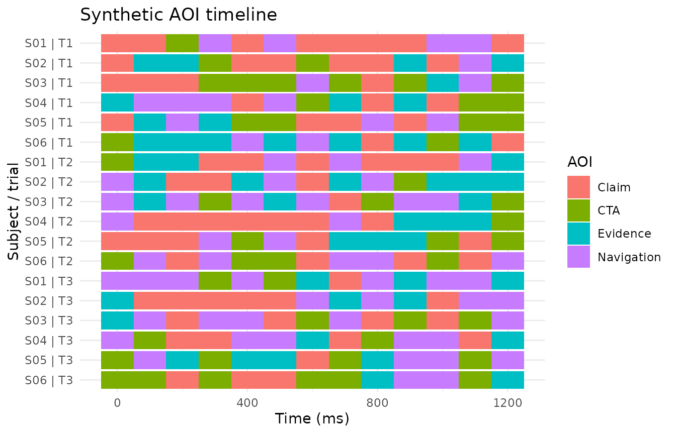
plot_gazepoint_aoi_timeline() provides a compact
scarf-style view of AOI state over time.
plot_gazepoint_aoi_timeline(
  aoi_demo,
  aoi_col = 'aoi',
  time_col = 'time_ms',
  subject_col = 'subject_id',
  trial_col = 'trial_id',
  title = 'Synthetic AOI timeline',
  x_label = 'Time (ms)'
)
Scanpath plot
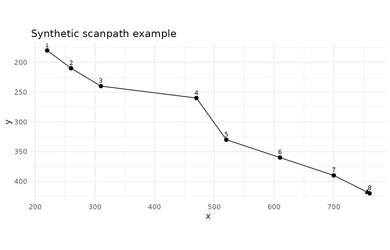
plot_gazepoint_scanpath() connects fixation coordinates
in temporal order.
plot_gazepoint_scanpath(
  fix_demo,
  x_col = 'x',
  y_col = 'y',
  group_cols = c('subject_id', 'trial_id'),
  time_col = 'start_time_ms',
  fixation_index_col = 'fixation_index',
  reverse_y = TRUE,
  title = 'Synthetic scanpath example'
)
Time-varying effect plot
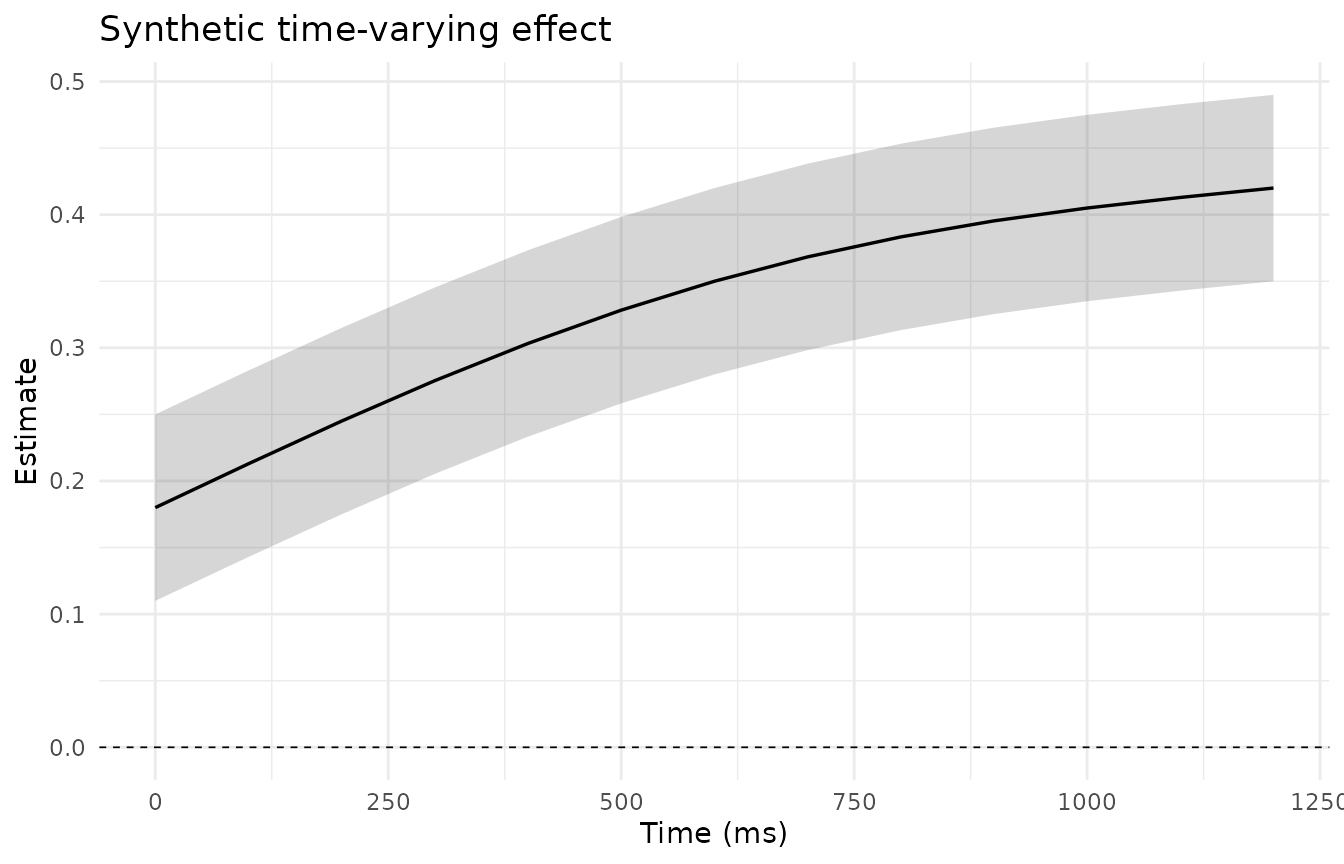
plot_gazepoint_time_varying_effect() visualises a
time-varying estimate and interval.
plot_gazepoint_time_varying_effect(
  effect_demo,
  time_col = 'time_ms',
  estimate_col = 'estimate',
  lower_col = 'lower',
  upper_col = 'upper',
  title = 'Synthetic time-varying effect',
  x_label = 'Time (ms)',
  y_label = 'Estimate'
)
Model residual diagnostics
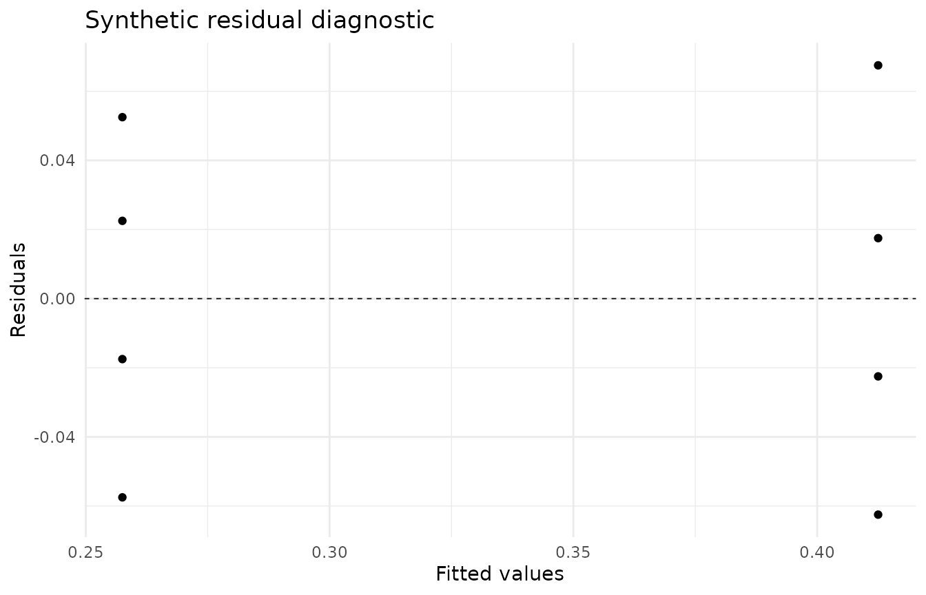
plot_gazepoint_model_residuals() gives a compact
residual diagnostic for fitted models.
plot_gazepoint_model_residuals(
  model = model_fit,
  title = 'Synthetic residual diagnostic'
)
Sequence and scanpath summaries
The extension layer also includes lightweight tabular sequence summaries.
compute_gazepoint_aoi_entropy(
  aoi_demo,
  aoi_col = 'aoi',
  group_cols = c('subject_id', 'trial_id'),
  time_col = 'time_ms',
  collapse_repeats = TRUE
) |> head()
#>   subject_id trial_id n_observations n_aoi spatial_entropy spatial_entropy_norm
#> 1        S01       T1              8     3        1.405639            0.8868595
#> 2        S02       T1             10     4        1.846439            0.9232197
#> 3        S03       T1              9     4        1.836592            0.9182958
#> 4        S04       T1             10     4        1.970951            0.9854753
#> 5        S05       T1             10     4        1.970951            0.9854753
#> 6        S06       T1             11     4        1.858555            0.9292776
#>   n_transitions n_transition_types transition_entropy transition_entropy_norm
#> 1             7                  4           1.842371               0.9211855
#> 2             9                  7           2.725481               0.9708358
#> 3             8                  6           2.500000               0.9671320
#> 4             9                  8           2.947703               0.9825676
#> 5             9                  8           2.947703               0.9825676
#> 6            10                  6           2.521928               0.9756150
#>   conditional_transition_entropy conditional_transition_entropy_norm
#> 1                      0.3935554                           0.2483058
#> 2                      0.8888889                           0.4444444
#> 3                      0.5943609                           0.2971805
#> 4                      1.0566417                           0.5283208
#> 5                      1.0566417                           0.5283208
#> 6                      0.7609640                           0.3804820
#>   entropy_status
#> 1             ok
#> 2             ok
#> 3             ok
#> 4             ok
#> 5             ok
#> 6             ok

compute_gazepoint_aoi_sequence_metrics(
  aoi_demo,
  aoi_col = 'aoi',
  group_cols = c('subject_id', 'trial_id'),
  time_col = 'time_ms'
) |> head()
#>   subject_id trial_id sequence_length n_aoi_visits n_unique_aoi
#> 1        S01       T1              13            8            3
#> 2        S02       T1              13           10            4
#> 3        S03       T1              13            9            4
#> 4        S04       T1              13           10            4
#> 5        S05       T1              13           10            4
#> 6        S06       T1              13           11            4
#>   transition_count revisit_count revisit_prop dominant_aoi first_aoi last_aoi
#> 1                7             5    0.6250000        Claim     Claim    Claim
#> 2                9             6    0.6000000        Claim     Claim Evidence
#> 3                8             5    0.5555556          CTA     Claim      CTA
#> 4                9             6    0.6000000   Navigation  Evidence      CTA
#> 5                9             6    0.6000000        Claim     Claim      CTA
#> 6               10             7    0.6363636     Evidence       CTA    Claim
#>   mean_run_length max_run_length sequence_status
#> 1        1.625000              4              ok
#> 2        1.300000              2              ok
#> 3        1.444444              3              ok
#> 4        1.300000              3              ok
#> 5        1.300000              2              ok
#> 6        1.181818              3              ok

compute_gazepoint_sequence_distance(
  c('Claim', 'Evidence', 'CTA'),
  c('Claim', 'CTA', 'Evidence')
)
#>   edit_distance normalized_distance sequence_a_length sequence_b_length
#> 1             2           0.6666667                 3                 3
#>   distance_status
#> 1              ok

compute_gazepoint_scanpath_similarity(
  aoi_demo[aoi_demo$subject_id %in% c('S01', 'S02') & aoi_demo$trial_id == 'T1', ],
  aoi_col = 'aoi',
  group_cols = 'subject_id',
  time_col = 'time_ms',
  collapse_repeats = TRUE
)
#>       sequence_a     sequence_b edit_distance normalized_distance similarity
#> 1 subject_id=S01 subject_id=S01             0                 0.0        1.0
#> 2 subject_id=S02 subject_id=S02             0                 0.0        1.0
#> 3 subject_id=S01 subject_id=S02             5                 0.5        0.5
#>   sequence_a_length sequence_b_length n_sequences similarity_status
#> 1                 8                 8           2                ok
#> 2                10                10           2                ok
#> 3                 8                10           2                ok