Example · Sensitivity analysis

Sampling sensitivity example

Sampling rate can change event representation, path geometry, and endpoint estimates. GazeAudit treats downsampling as a controlled perturbation of an existing study—not as a claim that a different physical tracker would have measured exactly the same trajectory.

Build a synthetic study

import numpy as np
import pandas as pd

from gazeaudit import GazeStudy

rng = np.random.default_rng(42)

rows = []
for participant in ["p01", "p02"]:
    for trial in [1, 2]:
        time_ms = np.arange(0.0, 2000.0, 1000.0 / 120.0)
        phase = np.linspace(0, 4 * np.pi, len(time_ms))
        x = 500 + 80 * np.sin(phase) + rng.normal(0, 2.0, len(time_ms))
        y = 400 + 45 * np.cos(phase) + rng.normal(0, 2.0, len(time_ms))
        rows.extend(
            {
                "participant": participant,
                "trial": trial,
                "timestamp": t,
                "x": x_i,
                "y": y_i,
            }
            for t, x_i, y_i in zip(time_ms, x, y, strict=True)
        )

frame = pd.DataFrame(rows)
study = GazeStudy(frame)

print(study.n_participants)
print(study.n_trials)
study.validate_time_order()

Downsample one stream family

from gazeaudit import downsample_gaze

study_60 = downsample_gaze(study, 60.0)
study_30 = downsample_gaze(study, 30.0)

print(len(study.data), len(study_60.data), len(study_30.data))

downsample_gaze() retains existing samples nearest to an ideal regular target grid. It does not interpolate gaze coordinates.

Define one common endpoint

For illustration, use the mean horizontal coordinate:

def endpoint(current_study):
    return float(current_study.data["x"].mean())

A real research endpoint should represent the scientific quantity you actually intend to stress-test—for example a condition contrast, path-rate contrast, dwell effect, or other predeclared scalar estimate.

Evaluate a sensitivity curve

from gazeaudit import sampling_sensitivity_curve

curve = sampling_sensitivity_curve(
    study,
    target_rates=[120, 90, 60, 45, 30],
    endpoint=endpoint,
)

print(curve)

The returned table includes:

• target_hz;
• n_rows retained after perturbation;
• retained_fraction relative to the original study;
• the common estimate.

Interpretation

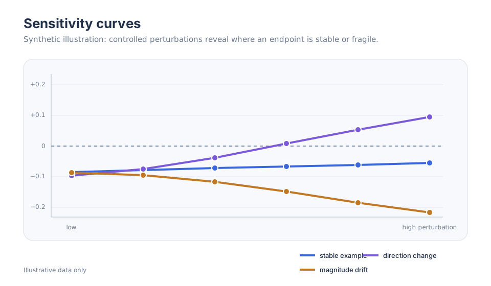
A sampling sensitivity curve asks whether the endpoint is stable when the same recorded stream is represented at lower controlled sampling rates.

It does not establish:

• cross-device equivalence;
• how a different tracker would behave physically;
• that interpolation could recover removed information;
• that one target rate is universally adequate for every endpoint.

Combine sampling with missingness

Sampling and missingness can interact. GazeAudit therefore provides separate missingness perturbation utilities rather than treating all row loss as equivalent to lower sampling rate.

Use inject_missingness(), missingness_mask(), or missingness_sensitivity_curve() when dropout or structured missingness is the scientific concern. Keep the perturbation mechanism explicit in the analysis record.

From example to study workflow

For formal robustness work:

1. justify the target rates before inspecting the resulting estimates;
2. preserve the original sampling information;
3. use one common endpoint at every target rate;
4. report retained sample fractions alongside endpoint changes;
5. keep sampling perturbation conceptually separate from measurement-error and missingness assumptions;
6. archive the complete curve, not only the most reassuring rate.

The frozen Pedrotti/de Chambrier case study provides an example where sampling and missingness sensitivity produced the canonical outcome materially_fragile; see the validation matrix for the provenance boundary.