End-to-end EDA research workflow
Run the complete workflow
The repository contains an executable Python-native companion at examples/hands-on/end-to-end-eda-research.py. It is executed by documentation CI, so the documented path is checked against the package rather than maintained as untested pseudocode. The separate examples/tutorials/ directory remains the frozen 26 R-companion tutorial surface.
The research question this workflow answers
Use this route when you have a continuous GSR/EDA channel and want to obtain descriptive electrodermal components and candidate SCR-like events while preserving the evidence needed to review the analysis. The workflow does not infer emotion, stress, preference, deception, diagnosis, or causal psychological response.
graph LR
  A[Load data] --> B[Audit units + activity]
  B --> C[Audit timing + quality]
  C --> D{Measurement ready?}
  D -- no --> X[Review mapping / exclusions]
  D -- yes --> E[Decompose EDA]
  E --> F[Detect candidate SCR events]
  F --> G[Inspect plots]
G --> H[Export tables + methods evidence]Inputs
The runnable example expects these demonstration columns:
| Column | Role |
|---|---|
participant_id |
grouping unit |
TIME |
analysis time column |
GSR_US |
conductance signal |
HR, IBI, LPMM |
additional channels used only in the initial activity audit |
For your own data, do not rename a column merely to make the example run. First establish what the vendor/export column actually measures, its units, its timebase, and whether it is raw or derived.
Stage 1 — load without destroying provenance
import gpbiometricspy as gp

raw = (
    gp.load_kiosk_demo(participants=["synthetic_kiosk_p001"])
    .copy()
    .iloc[:1800]
    .reset_index(drop=True)
)
With a study export, replace only the loading step, for example with the package importer appropriate to your file. Keep the original file name, participant/session identifiers, and untouched source file outside the derived-output directory.
Output: one in-memory table plus a traceable reference to the source.
Stage 2 — establish measurement readiness
Run unit, signal-activity, timing, quality, and artifact audits before decomposition:
groups = ["participant_id"]

units = gp.audit_gazepoint_gsr_units(raw, gsr_col="GSR_US")
activity = gp.audit_gazepoint_signal_activity(
    raw,
    signal_cols=["GSR_US", "HR", "IBI", "LPMM"],
    group_cols=groups,
)
time_resets = gp.audit_gazepoint_time_resets(
    raw,
    time_col="TIME",
    group_cols=groups,
)
quality = gp.audit_gazepoint_gsr_quality(raw, value_column="GSR_US")
artifacts = gp.audit_gazepoint_eda_artifacts(
    raw,
    signal_col="GSR_US",
    time_col="TIME",
    group_cols=groups,
)
Continue only when you can justify
- what
GSR_USrepresents and in which units; - that the signal is present and sufficiently variable for the intended descriptive analysis;
- which clock/time column is being used;
- whether resets, large gaps, missingness, flatline periods, or artifacts require exclusion or segmentation;
- which participant/session grouping defines an independent recording unit.
If these points are unresolved, the correct next step is review, not feature extraction.
Stage 3 — create explicit tonic and phasic components
decomposition = gp.decompose_gazepoint_eda(
    raw,
    signal_col="GSR_US",
    time_col="TIME",
    group_cols=groups,
    window_size=31,
    output_prefix="eda",
)
This produces eda_tonic and eda_phasic columns. The package's deterministic decomposition is a transparent descriptive workflow. For confirmatory electrodermal decomposition where a specialised method is scientifically required, use or cross-check an appropriate biosignal toolbox and report that choice.
Output: original rows plus explicit decomposition columns and stored settings/overview metadata.
Stage 4 — detect candidate SCR-like events
scr = gp.detect_gazepoint_scr_events(
    decomposition,
    phasic_col="eda_phasic",
    signal_col="GSR_US",
    time_col="TIME",
    group_cols=groups,
    threshold=None,
    min_peak_distance=10,
)
With threshold=None, the detector derives a local threshold from the phasic signal. The returned object includes an overview, an events table, a group summary, and the settings used.
Treat these as candidate waveform events, not direct psychological labels.
Stage 5 — inspect the evidence visually
decomposition_plot = gp.plot_gazepoint_eda_decomposition(
    decomposition,
    time_col="TIME",
    signal_cols=["GSR_US", "eda_tonic", "eda_phasic"],
    group_cols=groups,
    title="Observed, tonic and phasic EDA",
)

scr_plot = gp.plot_gazepoint_scr_events(
    decomposition,
    scr["events"],
    time_col="TIME",
    signal_col="GSR_US",
    phasic_col="eda_phasic",
    group_cols=groups,
    title="Candidate SCR events",
)
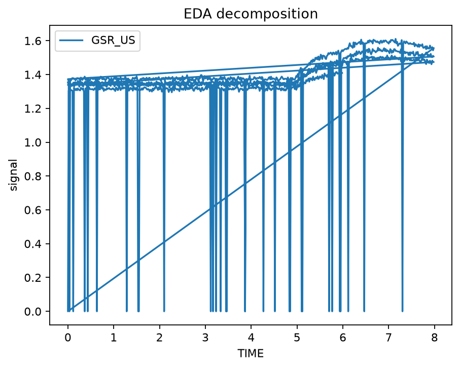
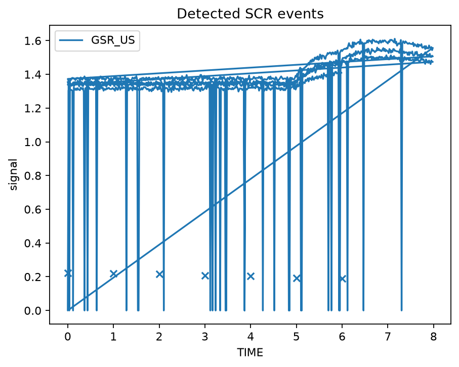
A plot is a diagnostic record, not decoration. Retain it with the output used for analysis.
Stage 6 — produce reporting evidence
checklist = gp.create_gazepoint_biometrics_checklist(raw)
methods_text = gp.create_gazepoint_biometrics_methods_text(checklist=checklist)
The checklist exposes active channels, missingness and basic quality evidence. The methods-text helper provides a reproducible starting point; it does not replace study-specific reporting of sampling, exclusions, preprocessing settings, experimental timing, or statistical analysis.
Stage 7 — export a reviewable analysis bundle
Run the checked example from the repository root:
The example writes:
outputs/eda-research/
├── eda_decomposition.csv
├── scr_events.csv
├── scr_group_summary.csv
├── analysis_checklist_overview.csv
├── methods_text.txt
├── end-to-end-eda-research-01.png
└── end-to-end-eda-research-02.png
The console also emits a small JSON PASS record describing the objects produced. This same executable is run by the documentation validator.
Replace the demonstration with your own export
Change the workflow in this order:
- Input mapping: load your file and identify participant/session, time, and EDA columns.
- Unit/time audit: verify units and observed timing before changing detector settings.
- QC rule: define exclusions or segmentation rules before inspecting condition effects.
- Decomposition: justify the method and window/settings for the scientific purpose.
- Event definition: predeclare threshold/window rules when event counts are inferentially important.
- Experimental alignment: only add stimulus-locked windows after clocks and event markers are defensible.
- Statistics: aggregate/model at the unit implied by the design; do not treat time samples as independent participants.
- Reporting: retain package version, source identity, settings, QC tables, exclusions, plots and analysis outputs.
Completion criteria
A workflow is report-ready when another researcher can determine:
- what was measured;
- which rows/participants were retained and why;
- which timebase was used;
- which transformation and event settings were applied;
- what the derived event table represents;
- which plots were inspected;
- which package/version produced the output;
- which claims are descriptive versus inferential.
Continue
- Hands-on EDA research guide — detailed teaching version of every step.
- Runnable end-to-end example — shortest copy-paste route.
- Validate a new dataset — use before substituting private study data.
- Reporting and reproducibility — publication-oriented evidence checklist.