EDA and SCR visual diagnostics • gpbiometrics

Purpose

This article demonstrates a plot-rich visual diagnostics workflow for electrodermal activity (EDA), galvanic skin response (GSR), and candidate skin conductance responses (SCRs) in gpbiometrics projects.

The workflow is intentionally diagnostic. The figures show signal continuity, unit/range checks, tonic-phasic separation, candidate event marking, response-window summaries, threshold sensitivity, and compact report-style displays. They should not be interpreted as direct evidence of emotion, stress, attention, workload, health status, clinical state, diagnosis, or psychological response.

Synthetic EDA/GSR stream

The example uses synthetic data so that the article is reproducible and does not depend on private recordings.

alpha_scr <- function(time_s, onset_s, amplitude, rise = 1.1, decay = 3.4) {
  x <- pmax(0, time_s - onset_s)
  response <- amplitude * (exp(-x / decay) - exp(-x / rise))
  response[x <= 0] <- 0
  response
}

participants <- sprintf("P%02d", 1:8)
trials <- seq_len(10)
samples_per_trial <- 360
time_s <- seq(0, 24, length.out = samples_per_trial)

trial_grid <- expand.grid(
  participant_id = participants,
  trial_id = trials,
  KEEP.OUT.ATTRS = FALSE,
  stringsAsFactors = FALSE
)

make_trial <- function(participant_id, trial_id) {
  condition <- ifelse(trial_id %% 2 == 0, "dense", "simple")
  participant_shift <- match(participant_id, participants) / 30
  trial_shift <- trial_id / 120
  tonic <- 1.2 + participant_shift + trial_shift + 0.08 * sin(2 * pi * time_s / 24)
  event_onsets <- c(4, 11, 18)
  amplitude_base <- ifelse(condition == "dense", 0.16, 0.11)
  amplitudes <- amplitude_base + rnorm(length(event_onsets), 0, 0.015)
  phasic <- Reduce(`+`, Map(function(onset, amp) alpha_scr(time_s, onset, amp), event_onsets, amplitudes))
  gsr_us <- tonic + phasic + rnorm(length(time_s), 0, 0.015)
  missing <- runif(length(time_s)) < ifelse(condition == "dense", 0.012, 0.007)
  gsr_us[missing] <- NA_real_
  data.frame(
    participant_id = participant_id,
    trial_id = trial_id,
    condition = condition,
    time_s = time_s,
    gsr_us = gsr_us,
    tonic_true = tonic,
    phasic_true = phasic,
    stringsAsFactors = FALSE
  )
}

eda <- do.call(
  rbind,
  Map(make_trial, trial_grid$participant_id, trial_grid$trial_id)
)

head(eda)
#>       participant_id trial_id condition     time_s   gsr_us tonic_true
#> P01.1            P01        1    simple 0.00000000 1.237740   1.241667
#> P01.2            P01        1    simple 0.06685237 1.227188   1.243067
#> P01.3            P01        1    simple 0.13370474 1.227325   1.244466
#> P01.4            P01        1    simple 0.20055710 1.249163   1.245865
#> P01.5            P01        1    simple 0.26740947 1.244250   1.247263
#> P01.6            P01        1    simple 0.33426184 1.222970   1.248658
#>       phasic_true
#> P01.1           0
#> P01.2           0
#> P01.3           0
#> P01.4           0
#> P01.5           0
#> P01.6           0

GSR signal trace

A single-trial trace is useful for checking continuity, missing stretches, range, and gross artifacts before event extraction.

one_trial <- eda[eda$participant_id == "P01" & eda$trial_id == 2, ]

plot(
  one_trial$time_s,
  one_trial$gsr_us,
  type = "l",
  xlab = "Time (s)",
  ylab = "Conductance (uS)",
  main = "GSR signal trace"
)

Synthetic GSR trace for one participant-trial segment.

Unit and range check

A range plot helps identify unusual scaling or unit-conversion problems. This is a technical plausibility check, not a substantive result.

hist(
  eda$gsr_us,
  breaks = 30,
  xlab = "Conductance (uS)",
  main = "GSR unit and range check"
)
abline(v = median(eda$gsr_us, na.rm = TRUE), lty = 2)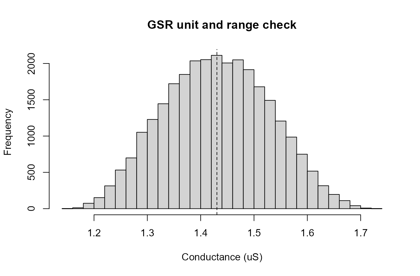

Synthetic GSR conductance range check.

Tonic-phasic decomposition

The example below uses a simple moving-average decomposition for visualization. In formal workflows, the decomposition method and parameters should be documented.

smooth_tonic <- stats::filter(one_trial$gsr_us, rep(1 / 51, 51), sides = 2)
smooth_tonic <- as.numeric(smooth_tonic)
smooth_tonic[is.na(smooth_tonic)] <- approx(
  x = which(!is.na(smooth_tonic)),
  y = smooth_tonic[!is.na(smooth_tonic)],
  xout = which(is.na(smooth_tonic)),
  rule = 2
)$y

phasic_est <- one_trial$gsr_us - smooth_tonic

op <- par(mfrow = c(2, 1), mar = c(3.5, 4, 2.5, 1))
plot(one_trial$time_s, one_trial$gsr_us, type = "l", xlab = "Time (s)", ylab = "GSR (uS)", main = "Observed GSR and tonic estimate")
lines(one_trial$time_s, smooth_tonic, lty = 2)
plot(one_trial$time_s, phasic_est, type = "l", xlab = "Time (s)", ylab = "Phasic estimate", main = "Estimated phasic component")
abline(h = 0, lty = 2)

Synthetic tonic-phasic decomposition display.

par(op)

Candidate SCR event markers

Candidate event markers document the detection rule and provide a visual audit trail for later review.

event_onsets <- c(4, 11, 18)
candidate_events <- do.call(
  rbind,
  lapply(event_onsets, function(onset) {
    idx <- which(one_trial$time_s >= onset & one_trial$time_s <= onset + 5)
    peak_idx <- idx[which.max(phasic_est[idx])]
    data.frame(
      onset_s = onset,
      peak_s = one_trial$time_s[peak_idx],
      amplitude = phasic_est[peak_idx],
      stringsAsFactors = FALSE
    )
  })
)
candidate_events$latency_s <- candidate_events$peak_s - candidate_events$onset_s

plot(
  one_trial$time_s,
  phasic_est,
  type = "l",
  xlab = "Time (s)",
  ylab = "Phasic estimate",
  main = "Candidate SCR events"
)
abline(h = 0, lty = 2)
abline(v = candidate_events$onset_s, lty = 3)
points(candidate_events$peak_s, candidate_events$amplitude, pch = 16)
text(candidate_events$peak_s, candidate_events$amplitude, labels = seq_len(nrow(candidate_events)), pos = 3)

Synthetic candidate SCR event markers.

candidate_events
#>   onset_s    peak_s  amplitude latency_s
#> 1       4  5.214485 0.05919195 1.2144847
#> 2      11 11.565460 0.04345445 0.5654596
#> 3      18 20.256267 0.02969727 2.2562674

Latency and recovery summaries

Latency and recovery summaries are useful for checking event-window extraction. They should be reported as algorithmic summaries unless the study design supports stronger inference.

event_summary <- do.call(
  rbind,
  lapply(seq_len(nrow(trial_grid)), function(i) {
    condition <- ifelse(trial_grid$trial_id[i] %% 2 == 0, "dense", "simple")
    amplitude_base <- ifelse(condition == "dense", 0.16, 0.11)
    data.frame(
      participant_id = trial_grid$participant_id[i],
      trial_id = trial_grid$trial_id[i],
      condition = condition,
      event = seq_along(event_onsets),
      onset_s = event_onsets,
      amplitude = pmax(0.02, amplitude_base + rnorm(length(event_onsets), 0, 0.025)),
      latency_s = pmax(0.4, 1.6 + rnorm(length(event_onsets), 0, 0.25)),
      recovery_s = pmax(1.0, 4.2 + rnorm(length(event_onsets), 0, 0.55)),
      stringsAsFactors = FALSE
    )
  })
)

op <- par(mfrow = c(1, 2), mar = c(4, 4, 3, 1))
boxplot(latency_s ~ condition, data = event_summary, xlab = "Synthetic condition", ylab = "Latency (s)", main = "SCR latency")
boxplot(recovery_s ~ condition, data = event_summary, xlab = "Synthetic condition", ylab = "Recovery time (s)", main = "SCR recovery")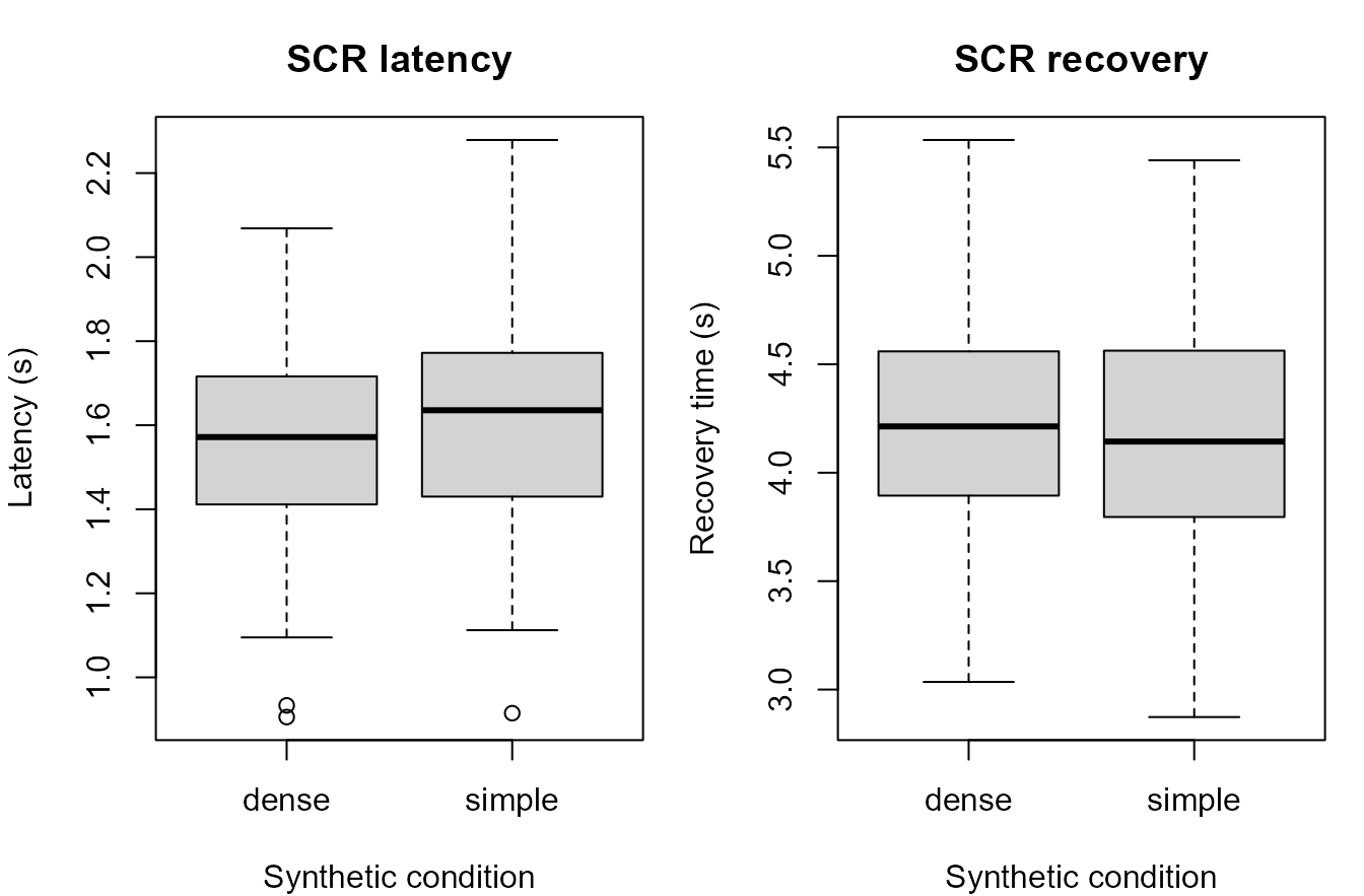

Synthetic SCR latency and recovery summaries.

par(op)

Threshold sensitivity

Threshold sensitivity plots show how candidate-response counts change when the amplitude threshold changes.

thresholds <- seq(0.04, 0.20, by = 0.02)
sens <- do.call(
  rbind,
  lapply(thresholds, function(th) {
    aggregate(
      event_summary$amplitude >= th,
      by = list(condition = event_summary$condition),
      FUN = mean
    ) |>
      transform(threshold = th)
  })
)
names(sens)[2] <- "detection_rate"

simple <- sens[sens$condition == "simple", ]
dense <- sens[sens$condition == "dense", ]

plot(
  simple$threshold,
  simple$detection_rate * 100,
  type = "b",
  ylim = c(0, 100),
  xlab = "Amplitude threshold",
  ylab = "Candidate events retained (%)",
  main = "SCR threshold sensitivity"
)
lines(dense$threshold, dense$detection_rate * 100, type = "b", pch = 17, lty = 2)
legend("topright", legend = c("simple", "dense"), lty = c(1, 2), pch = c(1, 17), bty = "n")

Synthetic SCR threshold sensitivity display.

Compact EDA/SCR visual diagnostics dashboard

A compact dashboard can combine range, signal, event, and threshold diagnostics for review or supplementary reporting.

op <- par(mfrow = c(2, 2), mar = c(4, 4, 3, 1))

hist(eda$gsr_us, breaks = 25, xlab = "Conductance (uS)", main = "Range check")

plot(one_trial$time_s, one_trial$gsr_us, type = "l", xlab = "Time (s)", ylab = "GSR (uS)", main = "Trace")

plot(one_trial$time_s, phasic_est, type = "l", xlab = "Time (s)", ylab = "Phasic", main = "Candidate SCRs")
points(candidate_events$peak_s, candidate_events$amplitude, pch = 16)

plot(simple$threshold, simple$detection_rate * 100, type = "b", ylim = c(0, 100), xlab = "Threshold", ylab = "Retained (%)", main = "Sensitivity")
lines(dense$threshold, dense$detection_rate * 100, type = "b", pch = 17, lty = 2)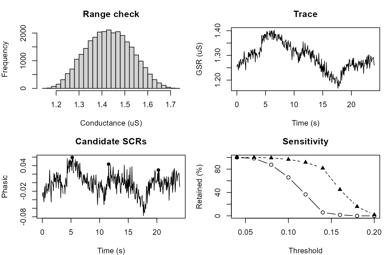

Compact synthetic EDA/SCR visual diagnostics dashboard.


par(op)

Relation to gpbiometrics helpers

The same reporting pattern can be paired with package-level helpers when project data use the expected column contracts.

task	representative_helpers
GSR unit audit	audit_gazepoint_gsr_units(); convert_gazepoint_gsr_to_conductance()
EDA decomposition	decompose_gazepoint_eda(); plot_gazepoint_eda_decomposition()
SCR event detection	detect_gazepoint_scr_events(); detect_gazepoint_scr_peaks(); plot_gazepoint_scr_events()
Latency and recovery summaries	compute_gazepoint_scr_latency(); extract_gazepoint_scr_recovery_times()
Threshold sensitivity	run_gazepoint_scr_threshold_sensitivity(); plot_gazepoint_scr_specification_curve()
Report outputs	create_gazepoint_qc_supplement(); create_gazepoint_biometrics_report_tables()

library(gpbiometrics)

gsr_units <- audit_gazepoint_gsr_units(
  biometric_data,
  gsr_col = "GSR"
)

eda_conductance <- convert_gazepoint_gsr_to_conductance(
  biometric_data,
  gsr_col = "GSR",
  output_col = "GSR_US"
)

eda_decomp <- decompose_gazepoint_eda(
  eda_conductance,
  eda_col = "GSR_US",
  time_col = "TIME_MS",
  participant_col = "participant_id",
  trial_col = "trial_id"
)

scr_events <- detect_gazepoint_scr_events(
  eda_decomp,
  phasic_col = "eda_phasic",
  time_col = "TIME_MS",
  participant_col = "participant_id",
  trial_col = "trial_id"
)

plot_gazepoint_eda_decomposition(eda_decomp)
plot_gazepoint_scr_events(eda_decomp, events = scr_events)

Reporting recommendation

For manuscripts, technical supplements, and reviewer-facing reports, describe these figures as EDA/GSR/SCR diagnostics, signal-processing checks, event-detection displays, threshold-sensitivity checks, and reproducibility outputs. Avoid stronger psychological, clinical, affective, workload-related, or stress-related interpretation unless supported by validation, controls, and modelling evidence.