AOI Perturbation and Uncertainty Analysis • eyeprocess

AOI Geometry Is an Analytical Assumption

AOI geometry is an analytical assumption. Small changes to a boundary can change whether a sample or fixation is counted as headline, image, claim, disclosure, CTA, outside, or ambiguous. The purpose of this workflow is not to find a preferred boundary. It asks whether a conclusion is stable under a declared set of defensible alternatives.

Use this analysis when observations cluster near boundaries, neighboring AOIs are close, or AOI size is comparable with expected spatial error. Do not use it as a substitute for calibration, coordinate-quality auditing, or preregistered stimulus design.

Synthetic advertising layout

The example is fully synthetic and intentionally small.

aois <- data.frame(
  aoi_id = c("headline", "image", "claim", "disclosure", "cta"),
  xmin = c(100, 300, 300, 300, 680),
  xmax = c(400, 700, 700, 700, 920),
  ymin = c(80, 190, 360, 500, 600),
  ymax = c(180, 340, 480, 590, 710)
)

set.seed(12)
centers <- data.frame(
  x = c(250, 500, 500, 500, 800),
  y = c(130, 270, 430, 560, 650),
  aoi = c("headline", "image", "claim", "disclosure", "cta")
)

rows <- list()
k <- 0L
for (participant in 1:8) {
  condition <- participant %% 2
  for (trial in 1:3) {
    for (j in seq_len(nrow(centers))) {
      n <- 5L + if (centers$aoi[j] == "disclosure" && condition == 1) 3L else 0L
      for (fix in seq_len(n)) {
        k <- k + 1L
        rows[[k]] <- data.frame(
          obs = k,
          participant = paste0("p", participant),
          trial = trial,
          condition = condition,
          x = rnorm(1, centers$x[j], 35),
          y = rnorm(1, centers$y[j], 22),
          duration = runif(1, .06, .18),
          time = j - 1 + (fix - 1) / 20
        )
      }
    }
  }
}
fixations <- do.call(rbind, rows)

AOI Perturbation Sensitivity Analysis

Pixels versus Degrees of Visual Angle

Degree-based perturbations require explicit display geometry and viewing distance. The workflow never silently converts units.

grid <- create_aoi_perturbation_grid(
  dilations = c(.25, .50, 1.00),
  erosions = .25,
  translations_x = .50,
  translations_y = .50,
  unit = "deg",
  include_baseline = TRUE,
  screen_width_px = 1024,
  screen_height_px = 768,
  viewing_distance = 60,
  physical_screen_size = c(53.1, 29.9),
  boundary_policy = "allow"
)

grid$table
#>   perturbation_id operation margin_x margin_y translation_x translation_y unit
#> 1        baseline  baseline     0.00     0.00           0.0           0.0  deg
#> 2 dilate_0.25_deg  dilation     0.25     0.25           0.0           0.0  deg
#> 3  dilate_0.5_deg  dilation     0.50     0.50           0.0           0.0  deg
#> 4    dilate_1_deg  dilation     1.00     1.00           0.0           0.0  deg
#> 5  erode_0.25_deg   erosion     0.25     0.25           0.0           0.0  deg
#> 6 shift_x_0.5_deg translate     0.00     0.00           0.5           0.0  deg
#> 7 shift_y_0.5_deg translate     0.00     0.00           0.0           0.5  deg
#>   seed boundary_policy
#> 1   NA           allow
#> 2   NA           allow
#> 3   NA           allow
#> 4   NA           allow
#> 5   NA           allow
#> 6   NA           allow
#> 7   NA           allow

The seven branches are the nominal geometry, three dilations, one erosion, one horizontal translation, and one vertical translation.

Propagating AOI Uncertainty Into Statistical Models

The perturbation framework does not choose an estimator. The model callback must explicitly report its estimator output, convergence flag, and model N; converged rows require finite estimates, standard errors, confidence limits, and a positive integer-valued N. Here the example uses the same base-R linear model for disclosure dwell in every branch.

model_callback <- function(features, assigned, spec) {
  target <- features[features$aoi == "disclosure", , drop = FALSE]
  condition_map <- unique(assigned[, c("participant", "condition")])
  target <- merge(target, condition_map, by = "participant", all.x = TRUE)

  fit <- stats::lm(dwell ~ condition, data = target)
  co <- summary(fit)$coefficients
  if (!"condition" %in% rownames(co)) stop("condition coefficient unavailable")

  estimate <- unname(co["condition", "Estimate"])
  se <- unname(co["condition", "Std. Error"])

  data.frame(
    term = "condition",
    estimate = estimate,
    SE = se,
    CI_low = estimate - 1.96 * se,
    CI_high = estimate + 1.96 * se,
    p_value = unname(co["condition", "Pr(>|t|)"]),
    model_converged = TRUE,
    N = stats::nobs(fit)
  )
}

Run geometry to inference

result <- run_aoi_sensitivity_analysis(
  fixations,
  aois,
  grid,
  x_col = "x",
  y_col = "y",
  observation_id_col = "obs",
  participant_col = "participant",
  trial_col = "trial",
  duration_col = "duration",
  time_col = "time",
  observation_level = "fixation",
  overlap_policy = "ambiguous",
  model_callback = model_callback,
  preprocessing_specification = list(duration_unit = "seconds"),
  event_detector = "synthetic_fixations",
  quality_rules = list(missing = "preserve", overlap = "ambiguous"),
  model_specification = list(
    family = "lm",
    outcome = "disclosure_dwell",
    predictor = "condition"
  )
)

summary <- summarise_aoi_sensitivity(result)
summary$assignment_stability
#>                 perturbation_id n_total n_comparable proportion_unchanged
#> baseline               baseline     636          636            1.0000000
#> dilate_0.25_deg dilate_0.25_deg     636          636            0.9827044
#> dilate_0.5_deg   dilate_0.5_deg     636          636            0.9748428
#> dilate_1_deg       dilate_1_deg     636          636            0.9591195
#> erode_0.25_deg   erode_0.25_deg     636          636            0.9811321
#> shift_x_0.5_deg shift_x_0.5_deg     636          636            1.0000000
#> shift_y_0.5_deg shift_y_0.5_deg     636          636            0.9559748
#>                 proportion_newly_assigned proportion_lost proportion_reassigned
#> baseline                       0.00000000      0.00000000           0.000000000
#> dilate_0.25_deg                0.01729560      0.00000000           0.000000000
#> dilate_0.5_deg                 0.02515723      0.00000000           0.000000000
#> dilate_1_deg                   0.03144654      0.00000000           0.009433962
#> erode_0.25_deg                 0.00000000      0.01886792           0.000000000
#> shift_x_0.5_deg                0.00000000      0.00000000           0.000000000
#> shift_y_0.5_deg                0.01886792      0.02515723           0.000000000
summary$inference_stability
#>                term n_models n_converged convergence_proportion
#> condition condition        7           7                      1
#>           same_sign_proportion median_estimate min_estimate max_estimate
#> condition                    1       0.3151472    0.2942975    0.3198195
#>           median_CI_width median_N min_N max_N
#> condition       0.2268699       24    24    24

Interpreting AOI Assignment Stability

The assignment table distinguishes unchanged observations, newly assigned observations, lost assignments, AOI-to-AOI reassignment, missing comparisons, and explicit overlap ambiguity. Missing coordinates are not converted to outside-AOI observations.

Fixation and sample input

The same geometry and assignment engine supports fixation-centroid and sample-level input. Declare observation_level = "fixation" or "sample". Output always contains universal observation counts/timing; fixation-specific fields are populated only for fixation input and sample counts only for sample input. This prevents sample rows from being reported as fixation counts.

Zero is not missing

Feature recomputation preserves the complete declared AOI universe within each observed participant/trial group. A zero observation_count means valid observations were available but none were assigned to that AOI; fixation_count or sample_count is populated only at the matching observation level. If a group has no valid AOI assignment opportunity, counts and inspection remain missing rather than being coerced to zero. Missing assigned durations make dwell missing, and first-observation timing is never inferred from row order.

Visual diagnostics

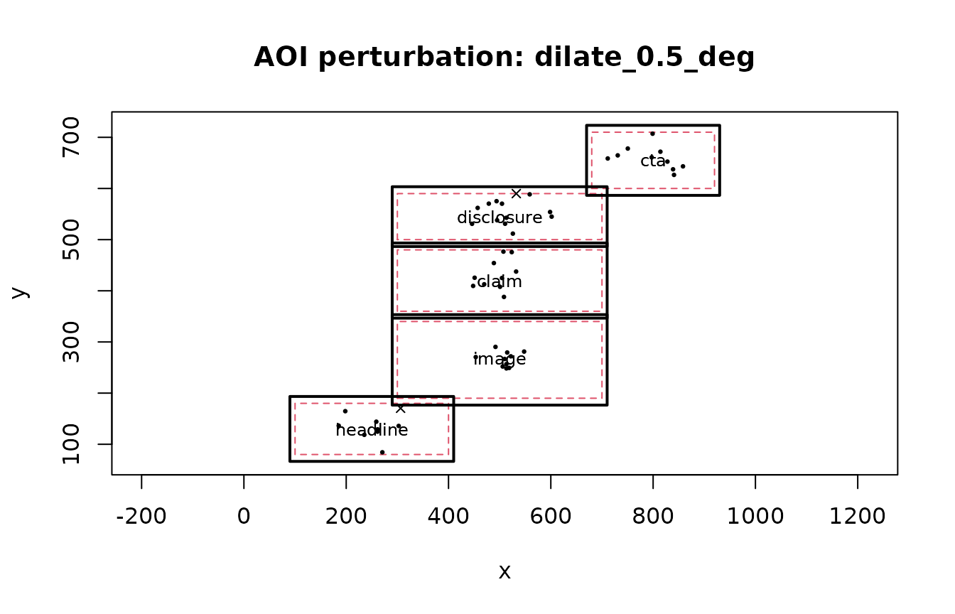
plot_aoi_perturbations(
  result,
  perturbation_id = "dilate_0.5_deg",
  data = fixations[seq(1, nrow(fixations), by = 12), ],
  x_col = "x",
  y_col = "y"
)

plot_aoi_assignment_stability(result)

plot_aoi_coefficient_stability(result, "condition")

Plot-to-question map

Visual	Function	Scientific question	Report with
Perturbed geometry	`plot_aoi_perturbations()`	Which observations cross a boundary when geometry changes?	perturbation ID, units, overlap/boundary policy
Assignment stability	`plot_aoi_assignment_stability()`	How much of the measurement mapping changes?	unchanged/new/lost/reassigned proportions
Coefficient stability	`plot_aoi_coefficient_stability()`	Does the same model change materially?	coefficient/interval range, convergence, model `N`
Robustness surface	`plot_aoi_robustness_surface()`	Where does sensitivity concentrate across two-dimensional perturbations?	both perturbation axes and the plotted stability metric

The robustness-surface plot is most useful when the analysis plan includes a two-dimensional perturbation grid. Do not construct a surface after seeing results merely to locate a favorable region.

surface_pairs <- as.matrix(expand.grid(
  margin_x = c(-.25, 0, .25, .50),
  margin_y = c(-.25, 0, .25, .50)
))
surface_grid <- create_aoi_perturbation_grid(
  anisotropic = surface_pairs,
  unit = "deg",
  include_baseline = TRUE,
  screen_width_px = 1024,
  screen_height_px = 768,
  viewing_distance = 60,
  physical_screen_size = c(53.1, 29.9),
  boundary_policy = "allow"
)
surface_result <- run_aoi_sensitivity_analysis(
  fixations, aois, surface_grid,
  x_col = "x", y_col = "y",
  observation_id_col = "obs",
  participant_col = "participant",
  trial_col = "trial",
  duration_col = "duration",
  time_col = "time",
  observation_level = "fixation"
)
plot_aoi_robustness_surface(surface_result)

The coefficient plot should be interpreted together with the assignment plot. A result can have many reassigned fixations without reversing a coefficient, or can show high aggregate assignment stability while a model estimate remains sensitive.

Demonstrate a failure branch

Excessive erosion is retained as a failed branch rather than disappearing.

failure_grid <- create_aoi_perturbation_grid(erosions = 500)
failure_result <- apply_aoi_perturbation_grid(aois, failure_grid)
failure_result$audit
#>   perturbation_id    status
#> 1        baseline completed
#> 2    erode_500_px    failed
#>                                                 message geometry_hash
#> 1                                                  <NA>     25689-662
#> 2 Perturbation `erode_500_px` collapsed AOI `headline`.          <NA>

Model callbacks follow the same rule: an error is written to the failure table, and a row with model_converged = FALSE remains visible rather than being treated as a valid estimate.

AOI Robustness Decision Clinic

Interpret assignment and model stability together rather than treating one metric as a verdict.

Pattern	Interpretation	Recommended response
High assignment stability + stable coefficient	Stable within the declared envelope	Report the envelope and stability summaries; do not call this proof that the nominal AOI is correct
Low assignment stability + stable coefficient	Mapping changes but the model-level result is insensitive	Report reassignment matrices and model stability together
High assignment stability + unstable coefficient	A small subset of groups or observations may be influential	Inspect participant/trial/AOI summaries, intervals, convergence, and model `N`
Low assignment stability + unstable coefficient	The substantive result depends materially on AOI geometry	Describe the nominal result as geometry-sensitive
Failed branches	Part of the planned sensitivity design is non-evaluable	Retain failures and explain them; never shrink the denominator silently

Choose perturbation magnitudes from acquisition precision, display geometry, stimulus layout, or a preregistered rationale. Do not search for the margin that restores statistical significance.

Reporting example

We reran AOI assignment, feature extraction, and the prespecified model across the nominal geometry and defensible perturbations. We report reassignment patterns, coefficient ranges and intervals, convergence, and model-N variation. Failed branches remain in the audit trail. Stability frequencies describe robustness to the declared perturbation set and are not probabilities that the scientific conclusion is true.

Planning the sensitivity analysis before results

For a fillable preregistration-style template and API mapping, see the companion AOI Sensitivity Analysis Plan and Reporting Template article.

Record the AOI sensitivity plan before examining branch-specific model results. At minimum, state:

the nominal AOI source and geometry representation;
whether rows are samples or fixations;
the perturbation operations and exact values;
pixel or degree units and the display/viewing geometry when degrees are used;
overlap and screen-boundary policies;
the fixed statistical model specification;
how failed geometry, callback errors, and non-convergence will be retained and reported.

Do not widen, shrink, or selectively edit the perturbation grid because a particular branch changes statistical significance.

Troubleshooting AOI perturbation branches

Diagnose the earliest failing layer first: geometry -> assignment -> feature recomputation -> model callback.

Symptom	Inspect	Interpretation
Perturbation status is `failed`	`result$grid_result$audit`	Geometry could not be evaluated; keep the branch in the planned denominator
Many `__ambiguous__` assignments	perturbed AOIs and reassignment matrix	AOIs overlap under that perturbation; do not silently choose one
Many `__outside__` assignments	units, coordinate transform, AOI location	Layout/assignment mismatch, not automatically zero exposure
Count is zero	valid-observation denominator	Valid observations existed but none entered that AOI
Count is missing	missing-coordinate denominator	No valid assignment opportunity existed; do not coerce to zero
Callback failure	`result$failures`	Model branch is non-evaluable, not a valid null result
`model_converged = FALSE`	model table and estimator diagnostics	Retain the row but exclude it from converged-effect summaries
Model `N` changes	inference stability table	Case loss varies across branches and must be reported

A compact audit pattern is:

result$grid_result$audit[, c("perturbation_id", "status", "message")]
result$failures
result$models[, c("perturbation_id", "term", "model_converged", "N")]
assess_aoi_inference_stability(result, term = "condition")

The package does not reinterpret a geometry failure as a model result, a callback exception as non-significance, or missing assignment opportunity as a structural zero.

Reporting problematic branches

Of the planned AOI perturbations, all non-evaluable geometry and model branches were retained in the audit trail. Overlap ambiguity remained explicit, missing assignment opportunities were not converted to zero, and non-converged model rows were excluded from converged-effect summaries. Model-N variation was reported alongside coefficient and assignment stability.

This is a reporting template, not an empirical result.

Figure set for manuscripts and reviewer responses

A compact evidence set usually contains: (1) one geometry/reassignment figure, (2) assignment stability, and (3) coefficient stability. Add the two-dimensional robustness surface only when joint geometry changes are part of the prespecified sensitivity plan. Pair the figures with the branch audit, failure table, convergence summary, and model-N range rather than presenting plots without denominators.

Reporting AOI Robustness

For manuscript supplements, reviewer responses, or replication handoff, see the companion AOI Robustness Reporting Bundle article for a recommended file set, export pattern, privacy guidance, and API map.

cat(report_aoi_sensitivity(result))
#> ## AOI perturbation sensitivity analysis
#> 
#> Planned perturbations: 7; completed geometry branches: 7; geometry failures: 0; model callback failures: 0.
#> Median unchanged AOI assignment across completed perturbations: 0.981.
#> 
#> Model-level sensitivity is summarized by coefficient direction, magnitude, interval width, and convergence rather than significance alone.
#> - condition: 7/7 converged; same-sign frequency=1.000; median estimate=0.3151; range=[0.2943, 0.3198]; N range=[24, 24].
#> 
#> Interpretation: these quantities describe robustness to the declared AOI perturbations. They are not probabilities that the scientific conclusion is true.

A manuscript should report the nominal AOI source, coordinate system, observation level, perturbation operations and values, pixel-versus-degree units, screen geometry and viewing distance when degrees are used, overlap policy, screen-boundary policy, random seed for jitter, assignment denominators, recomputed features, model specification, coefficient/interval ranges, convergence, model-N variation, and handling of failed or non-converged branches.

Robustness frequencies are descriptive summaries conditional on the declared perturbation set. They are not probabilities that the scientific conclusion is true.

R/Python Scientific Parity

The R and Python implementations share the same perturbation IDs, outside and ambiguous labels, missing-coordinate semantics, unit requirements, failure records, model-convergence handling, and interpretation caveat. Both ship the same frozen two-AOI parity fixture.

Parity is semantic rather than byte-for-byte numerical identity. Base-R and NumPy random-number generators are allowed to produce different jitter coordinates from the same integer seed, provided each implementation is deterministic for its own seed and records that seed. Plot objects are also language-native: base R graphics in eyeprocess and Matplotlib axes in eyeprocesspy.

User-supplied model callbacks may use different statistical backends, so exact coefficient equality is not required unless the same estimator and numerical backend are deliberately used.

Limitations

Geometry perturbation does not replace calibration-error analysis.
It does not replace event-detector sensitivity analysis.
Exact concave-polygon buffering requires a dedicated geometry engine; the dependency-free core rejects concave dilation/erosion rather than silently approximating it.
Degree conversion inherits uncertainty in screen dimensions and viewing distance.
The perturbation envelope must be scientifically defensible; wider grids do not automatically provide stronger evidence.

API map

Use create_aoi_perturbation_grid() to declare branches, run_aoi_sensitivity_analysis() for the complete workflow, estimate_aoi_assignment_stability() for assignment robustness, assess_aoi_inference_stability() for coefficient/convergence/model-N summaries, and report_aoi_sensitivity() for a compact reporting draft.