Prior sensitivity and independent information: an analytical Bayesian example

A fully declared conjugate model

This self-contained, synthetic illustration uses a known-variance normal likelihood, not a multilevel gaze mediation model. Its purpose is to show that a fitted effect and its interval depend on both independent information and declared prior scale. It is not a claim about brms, hardware validity, Bayesian mediation identification, or data-based prior elicitation.

For independent observations y_i ~ Normal(mu, 1), take the prior mu ~ Normal(0, tau^2). The exact conjugate posterior has variance (n + 1/tau^2)^(-1) and mean sum(y)/(n + 1/tau^2). All uncertainty values below are model-conditional credible intervals, not frequency-calibrated confidence intervals.

set.seed(20261022)
y <- stats::rnorm(18, mean = 0.35, sd = 1)
prior_sd <- c(0.10, 0.25, 0.50, 1, 2.5, 5)
posterior_sd <- sqrt(1 / (length(y) + 1 / prior_sd^2))
posterior_mean <- sum(y) / (length(y) + 1 / prior_sd^2)
q <- stats::qnorm(0.975)
tab <- data.frame(prior_sd = prior_sd, posterior_mean = posterior_mean,
                  lower = posterior_mean - q * posterior_sd,
                  upper = posterior_mean + q * posterior_sd)
stopifnot(all(tab$lower <= tab$posterior_mean),
          all(tab$posterior_mean <= tab$upper))
tab

##   prior_sd posterior_mean      lower     upper
## 1     0.10     0.03171914 -0.1487102 0.2121484
## 2     0.25     0.11008406 -0.2260470 0.4462151
## 3     0.50     0.17012991 -0.2477358 0.5879956
## 4     1.00     0.19699252 -0.2526541 0.6466391
## 5     2.50     0.20610451 -0.2538238 0.6660329
## 6     5.00     0.20747550 -0.2539800 0.6689310

Figure 1. Analytical posterior intervals across prior scales

graphics::plot(tab$posterior_mean, seq_along(tab$prior_sd),
  xlim = range(c(tab$lower, tab$upper)), ylim = c(0.5, nrow(tab) + 0.5),
  pch = 19, col = "#24577B", yaxt = "n",
  xlab = "Conditional posterior location", ylab = "Prior SD",
  main = "Declared prior sensitivity")
graphics::axis(2, at = seq_along(tab$prior_sd),
               labels = format(tab$prior_sd), las = 1)
graphics::segments(tab$lower, seq_along(tab$prior_sd),
                   tab$upper, seq_along(tab$prior_sd),
                   lwd = 2, col = "#567B97")
graphics::abline(v = 0, lty = 3, col = "#8E8E8E")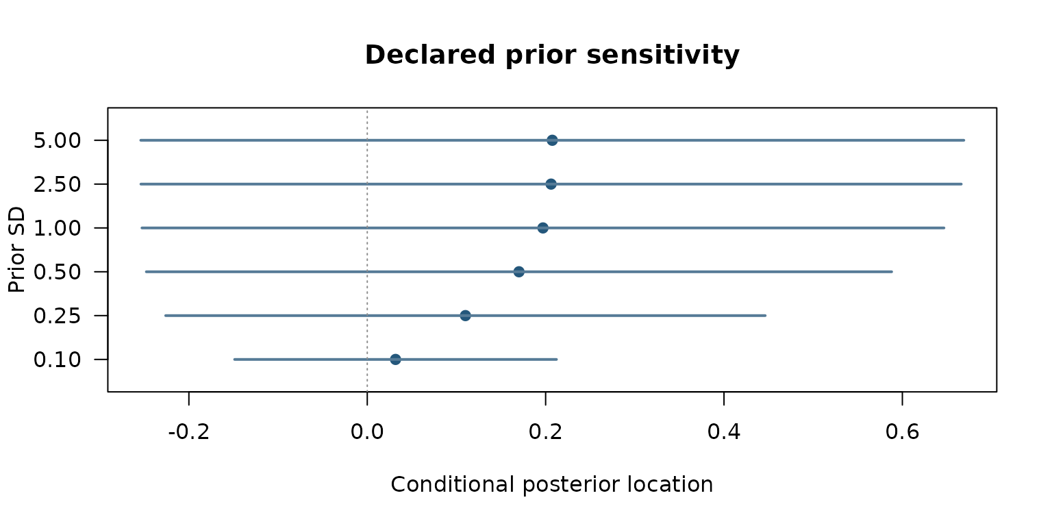

Synthetic normal-normal analytical posterior means and 95% equal-tailed credible intervals at declared prior scales. Not a posterior computation for the gp3bayes multilevel mediation API.

Figure 2. Likelihood and prior precision

prior_precision <- 1 / prior_sd^2
posterior_precision <- length(y) + prior_precision
graphics::plot(log10(prior_sd), prior_precision / posterior_precision,
  type = "b", pch = 19, col = "#B05E43",
  xaxt = "n", ylim = c(0, 1), xlab = "Prior standard deviation",
  ylab = "Prior fraction of total precision",
  main = "Independent information versus prior concentration")
graphics::axis(1, at = log10(prior_sd), labels = prior_sd)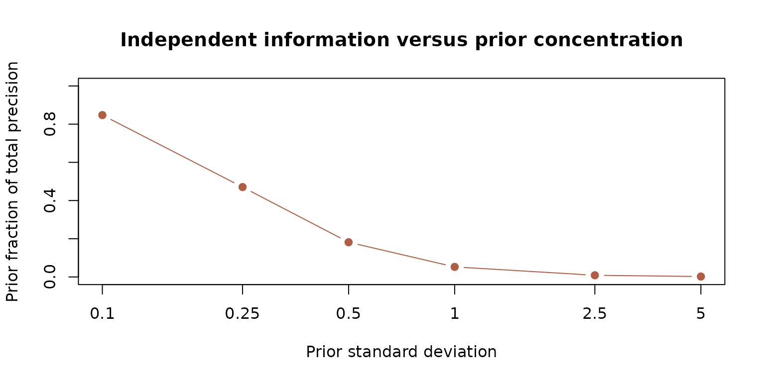

Exact posterior precision decomposition for the deliberately simple normal model; no uncertainty about the residual variance is propagated.

Limits and implications

The independence assumption, normal likelihood, known residual variance and single scalar parameter make this an elementary algebraic example rather than a validated workflow for gaze, SCR, pupil, participant heterogeneity, missingness or causal mediation. Posterior credible bounds are valid conditional on that declared model. Priors and sensitivity ranges must be justified by measurement scales and domain knowledge; an apparent stable interval is not a substitute for recovery, prior predictive checks, external reference data or conditional causal identification.

The more ambitious evidence-atlas, mediation-functional-form and uncertainty diagnostics remain in draft research PR #28, without a stable CRAN promotion. Current GitHub 0.6.0 and CRAN 0.5.0 are different publication lines.